K-Means and KNN

Posted on 2017-03-16 Edited on 2024-12-04 In ML Views: Word count in article: 12k Reading time ≈ 11 mins.

以简单的Iris数据集做测试，实现了K-means++聚类算法，并与sklearn中自带的KNN算法进行比较
标题本来是K-Means&KNN，把&改成了和，因为标题中出现特殊符号&会导致我的sitemap生成错误......

Introduction

K-Means is a simple partition-based clustering method. The problem it aims to solve is that given n samples (point set X), their feature vectors are projected into a high-dimensional space, and according to the spatial distribution, they can be roughly divided into several subspaces, with points in each subspace belonging to the same class. Now, it is necessary to calculate the class of each point. The basic idea is to randomly select k points (center point set C) as center points, and the remaining points self-organize: they join the team of the closest among the k center points, i.e., they are assigned to the same class as that center point. This way, k classes are formed. The process is repeated, and during this time, a loss evaluation is introduced, such as using the sum of the distances from each point in the class to the center point of that class as the evaluation indicator. The repetition stops when the indicator is less than a certain degree or when the change in the indicator is less than a certain degree
KNN is relatively simple and rough, its idea being similar to democratic voting. KNN does not train data; it selects a value K, and for each vector that needs to be predicted, it finds the K nearest points in the known category dataset. The category with the most points among these K points is the predicted category, i.e., it allows the K nearest points to the point to vote on the category of this point, and the category with the most votes is the category.

K-means++

k-means++ optimizes the selection of the initial k points on top of k-means. The original algorithm randomly selects k points, which is obviously too uncertain. A better scheme for selecting k points should be that they are as far apart from each other as possible, but not too far. As far apart as possible allows them to be as close as possible to the final ideal center point distribution; not too far is to prevent some erroneous points or outliers from being isolated as center points.
The algorithmic implementation first randomly selects the first center point from the set X, and then repeatedly performs the following process to select center points
- Calculate the distance from each point \(c_i\) to the already selected center point \(k_1,k_2...\) , select the smallest distance as the distance of \(c_i\) , and the significance of this distance is that when \(c_i\) is used as the next center point, it is at least this distance away from other center points
- Normalize the distance of \(c_1,c_2,c_3......\) and arrange it in a line
- The line has a length of 1, which is divided into many segments. The length of each segment represents the proportion of the distance of the point it represents in normalization; the greater the distance, the greater the proportion
- Select a random number between (0,1), and the point represented by the interval in which this number falls is the next centroid. Add it to the set of centroids C, and then repeat to find the next centroid
It can be seen that the likelihood of being randomly selected online increases with distance, which meets our requirements

K-Means code implementation

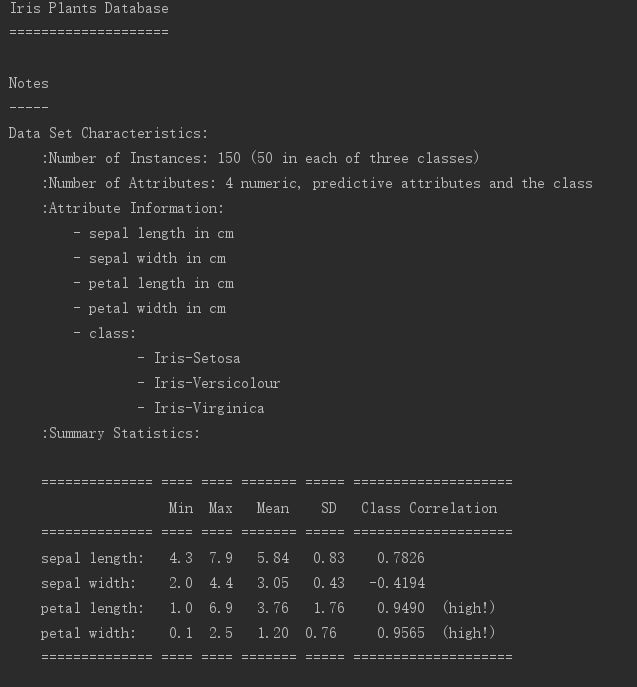
Data inspection

Iris is the Iris flower classification dataset, with 150 samples evenly divided into 3 classes, each sample having 4 attributes

Initialization of data

def init():
   iris = load_iris()
   X_train, X_test, y_train, y_test = train_test_split(iris.data, iris.target, test_size=0.25, random_state=33)
   ss = StandardScaler()
   X_train = ss.fit_transform(X_train)
   X_test = ss.fit_transform(X_test)
   return X_train, X_test, y_train, y_test, iris

k-means++ initialization of k points

D2 is the distance of each point (i.e., how far it is from other center points)
probs are normalized

cumprobs sum up the normalized probabilities, forming a line

        def initk(X_train, k):
            C = [X_train[0]]
            for i in range(1, k):
                D2 = scipy.array([min([scipy.inner(c - x, c - x) for c in C]) for x in X_train])
                probs = D2 / D2.sum()
                cumprobs = probs.cumsum()
                r = scipy.rand()
                for j, p in enumerate(cumprobs):
                    if r < p:
                        i = j
                        break
                C.append(X_train[i])
            return C
    

Loss Assessment
---------------

*   The sum of the squared distances from each point to the center of the class is used as the loss evaluation here
    
        def evaluate(C, X_train, y_predict):
           sum = 0
           for i in range(len(X_train)):
               c = C[y_predict[i]]
               sum += scipy.inner(c - X_train[i], c - X_train[i])
           return sum
        
    

Clustering
----------

*   After initializing k centroids, all points can be classified
    
*   Re-select the centroid for each class, here taking the average coordinates of all points in a class as the centroid coordinates
    
        def cluster(C, X_train, y_predict, k):
           sum = [0, 0, 0, 0] * k
           count = [0] * k
           newC = []
           for i in range(len(X_train)):
               min = 32768
               minj = -1
               for j in range(k):
                   if scipy.inner(C[j] - X_train[i], C[j] - X_train[i]) < min:
                       min = scipy.inner(C[j] - X_train[i], C[j] - X_train[i])
                       minj = j
               y_predict[i] = (minj + 1) % k
           for i in range(len(X_train)):
               sum[y_predict[i]] += X_train[i]
               count[y_predict[i]] += 1
           for i in range(k):
               newC.append(sum[i] / count[i])
           return y_predict, newC
        
    

Main Function
-------------

*   Compute the loss, update k centroids, and then re-cluster again
    
*   Repeat until the change in loss is less than 10%
    
*   Each iteration displays the old and new losses, showing the change in loss
    
*   Final output classification result
    
        def main():
           X_train, X_test, y_train, y_test, iris = init()
           k = 3
           total = len(y_train)
           y_predict = [0] * total
           C = initk(X_train, k)
           oldeval = evaluate(C, X_train, y_predict)
           while (1):
               y_predict, C = cluster(C, X_train, y_predict, k)
               neweval = evaluate(C, X_train, y_predict)
               ratio = (oldeval - neweval) / oldeval * 100
               print(oldeval, " -> ", neweval, "%f %%" % ratio)
               oldeval = neweval
               if ratio < 0.1:
                   break
        
           print(y_train)
           print(y_predict)
           n = 0
           m = 0
           for i in range(len(y_train)):
               m += 1
               if y_train[i] == y_predict[i]:
                   n += 1
           print(n / m)
           print(classification_report(y_train, y_predict, target_names=iris.target_names))
        
    

    # KNN code
    -   Just use KNeighborsClassifier
    ```Python
        from sklearn.datasets import load_iris
        from sklearn.preprocessing import StandardScaler
        from sklearn.neighbors import KNeighborsClassifier
        from sklearn.model_selection import train_test_split
        from sklearn.metrics import classification_report
    
    
        def init():
            iris = load_iris()
            X_train, X_test, y_train, y_test = train_test_split(iris.data, iris.target, test_size=0.25, random_state=33)
            ss = StandardScaler()
            X_train = ss.fit_transform(X_train)
            X_test = ss.fit_transform(X_test)
            return X_train, X_test, y_train, y_test, iris
    
    
        def KNN(X_train, X_test, y_train, y_test, iris):
            knc = KNeighborsClassifier()
            knc.fit(X_train, y_train)
            y_predict = knc.predict(X_test)
            print(knc.score(X_test, y_test))
            print(classification_report(y_test, y_predict, target_names=iris.target_names))
    
    
        def main():
            X_train, X_test, y_train, y_test, iris = init()
            KNN(X_train, X_test, y_train, y_test, iris)
    
        if __name__ == "__main__":
            main()
    

Predictive Results
==================

*   Indicator Description: For binary classification, the total number of four cases: correctly predicted as positive TP; correctly predicted as negative FN; incorrectly predicted as positive FP; incorrectly predicted as negative TN
    
    $$
    Precision:P=\frac{TP}{TP+FP} \\
    Recall:R=\frac{TP}{TP+FN} \\
    F1:\frac {2}{F_1}=\frac1P+\frac1R \\
    $$
    
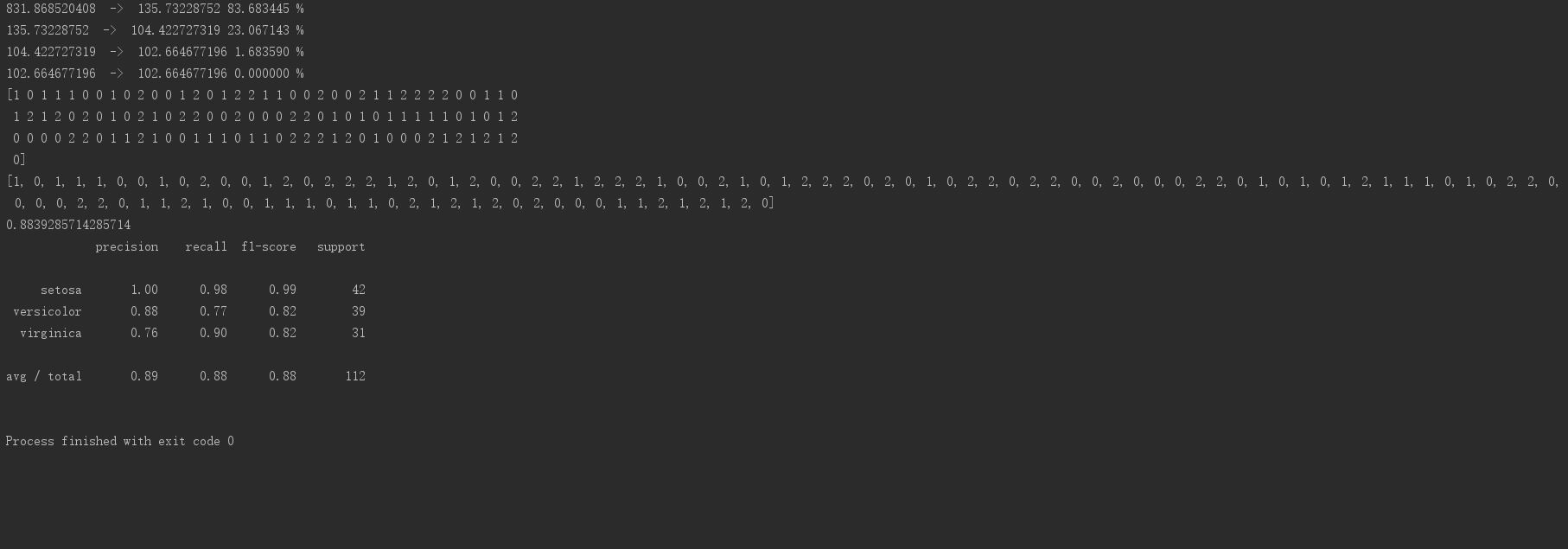
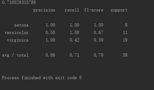
*   K-Means program output: Prediction accuracy: 88.39%, Average precision: 89%, Recall rate: 0.88, F1 score: 0.88 ![i0o1Ts.jpg](https://s1.ax1x.com/2018/10/20/i0o1Ts.jpg) 
    
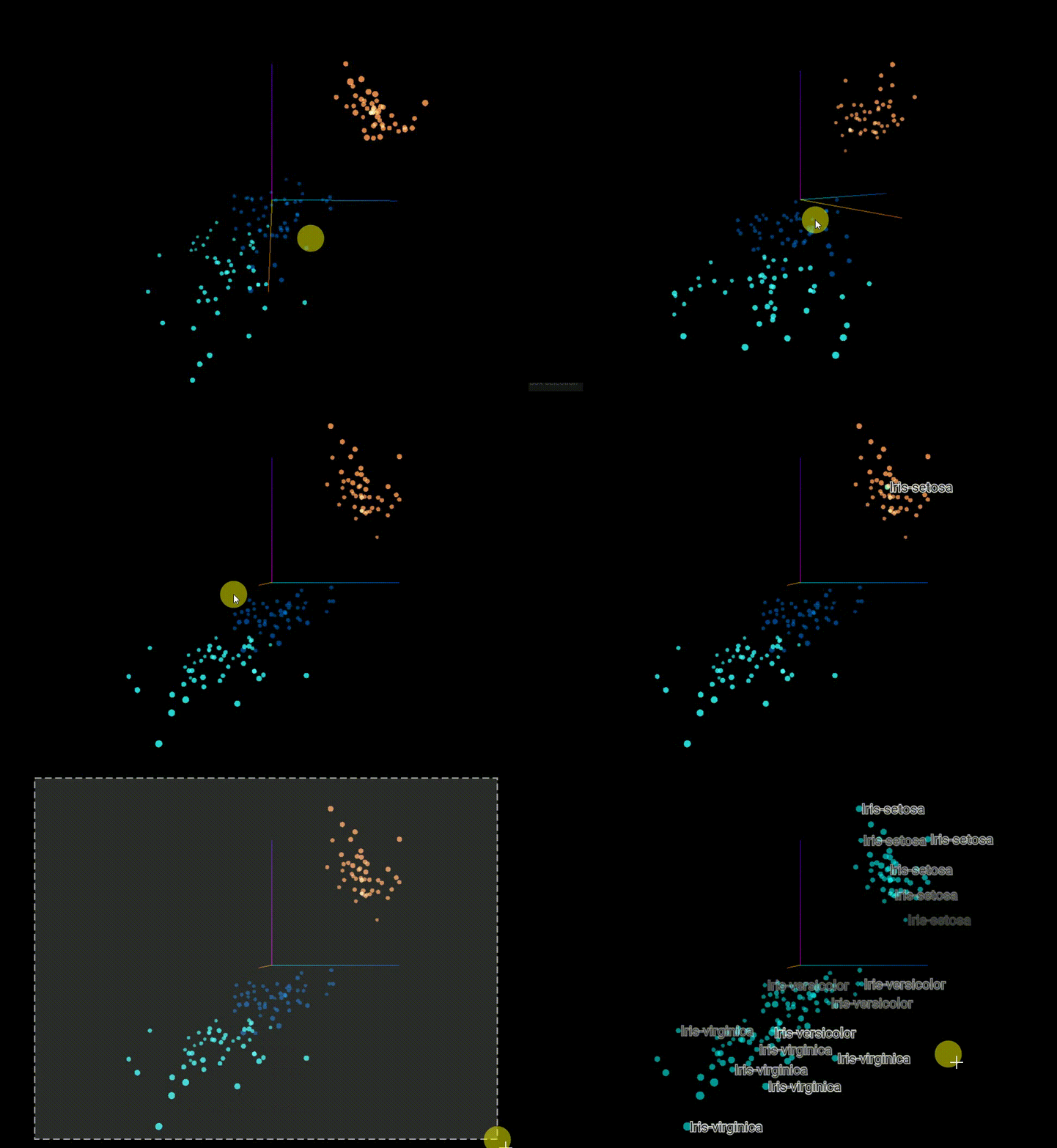
*   KNN program output: Prediction accuracy: 71.05%, Average precision: 86%, Recall rate: 0.71, F1 score: 0.70 ![i0oKOg.jpg](https://s1.ax1x.com/2018/10/20/i0oKOg.jpg) 
    
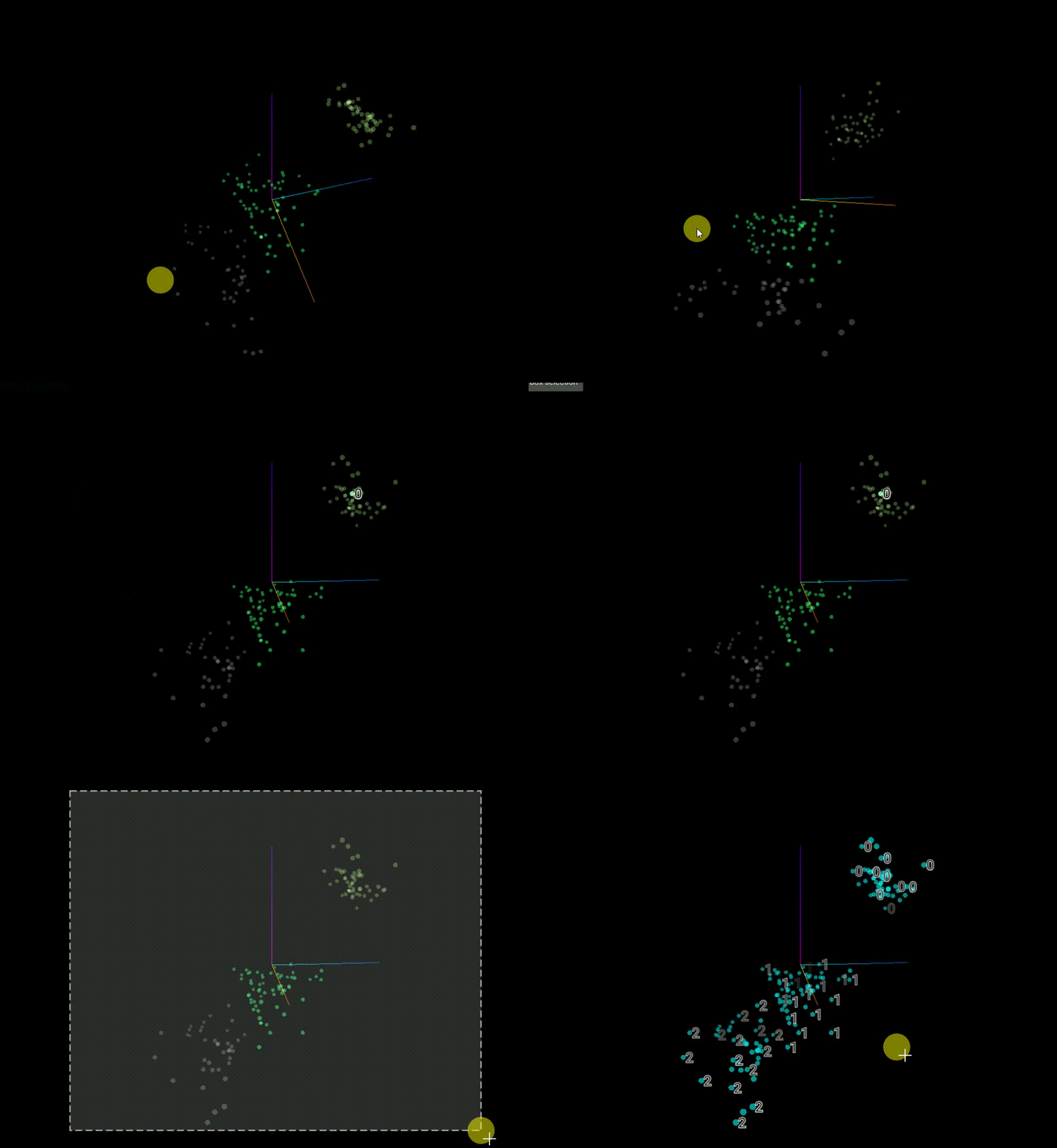
*   Original Classification: It can be seen that the dataset itself is spatially convenient for clustering segmentation ![i0oQmQ.gif](https://s1.ax1x.com/2018/10/20/i0oQmQ.gif) 
    
*   Predictive Classification ![i0o8kn.gif](https://s1.ax1x.com/2018/10/20/i0o8kn.gif) 
    

Improved
========

Unknown k situation
-------------------

*   Above is what we know about irises being divided into 3 categories; what if we don't know how many categories there are? After all, k-means is an unsupervised learning algorithm, which can be computed without labels. It is also highly possible that we do not know the number of natural labels, so how do we determine k?
*   A type of canopy algorithm
*   To be supplemented

Handling of empty classes
-------------------------

*   To be supplemented

Different distance calculation methods
--------------------------------------

*   To be supplemented

ANN algorithm
-------------


{% endlang_content %}

{% lang_content zh %}

# 简介

- K-Means是简单的基于划分的聚类方法，要解决的问题是，现在有n个样本(点集X)，将他们的特征向量投射到高维空间中，根据空间分布可以大致划分成几个子空间，每个子空间中的点属于同一类，现在需要计算出每个点所在的类，大致思想就是随机选择k个点(中心点集C)作为中心点，其余的点自己站队：离k个中心点里哪个点最近就站那个点的队，即和那个中心点划分到同一类中，这样就能形成k个类，重复上过程，期间引入一个损失评估，比如以各个类中的点到这个类中心点距离的和作为评估指标，当指标小于某一程度或者指标变化小于某一程度就停止重复
- KNN则比较简单粗暴，其思想类似于民主投票。KNN不训练数据，选定一个值K，对于每一个需要预测的向量，在已知类别的数据集中找到与这个向量最近的K，这K个点中拥有最多点个数的类别就是预测类别，即让离某个点最近的K个点投票决定这个点的类别，哪个类别的点票数多就是哪个类别

# K-means++

- k-means++在k-means上优化了初始k个点的选择。原始算法是随机取k个点，显然这样随机不确定性太大，比较好的k个点的选择方案应该是他们离彼此尽量远，但不能太远。尽量远，就能尽可能贴近最终理想中心点分布；不能太远，是为了防止将一些错误点孤立点作为中心点
- 算法上的实现是先随机从X集中取第一个中心点，之后反复以下过程取中心点
  - 计算每个点$c_i$到已经选出的中心点$k_1,k_2...$的距离，选取最小的一个距离作为$c_i$的距离，这个距离的意义即$c_i$作为下一个中心点时离其他中心点至少有多远
  - 将$c_1,c_2,c_3......$的距离归一化，并排成一条线
  - 这条线长度为1，分成了许多段，每一段的长度就代表了这一段所代表的点的距离在归一化中所占的比例，距离越大，比例越大
  - 在(0,1)之间随机取一个数，这个数所在的段区间所代表的点就是下一个中心点，将其加入中心点集C，接着重复找下一个中心点
- 可以看出，如果距离够远，在线上被随机抽到的可能越大，符合我们的需求

# K-Means代码实现

## 数据检视

- Iris是鸢尾花分类数据集，150个样本，均匀分成3类，每一个样本有4个属性
  ![i0otpV.jpg](https://s1.ax1x.com/2018/10/20/i0otpV.jpg)

## 初始化数据

- 初始化数据
  
  ```Python
  def init():
     iris = load_iris()
     X_train, X_test, y_train, y_test = train_test_split(iris.data, iris.target, test_size=0.25, random_state=33)
     ss = StandardScaler()
     X_train = ss.fit_transform(X_train)
     X_test = ss.fit_transform(X_test)
     return X_train, X_test, y_train, y_test, iris

## k-means++初始化k个点
-    D2是每个点的距离(即之前定义的里其他中心点至少有多远)
-    probs归一化
-    cumprobs将归一化的概率累加，排列成一条线
```Python
    def initk(X_train, k):
        C = [X_train[0]]
        for i in range(1, k):
            D2 = scipy.array([min([scipy.inner(c - x, c - x) for c in C]) for x in X_train])
            probs = D2 / D2.sum()
            cumprobs = probs.cumsum()
            r = scipy.rand()
            for j, p in enumerate(cumprobs):
                if r < p:
                    i = j
                    break
            C.append(X_train[i])
        return C

损失评估

在这里用每个类内点到中心点距离平方和的总和作为损失评估

def evaluate(C, X_train, y_predict):
   sum = 0
   for i in range(len(X_train)):
       c = C[y_predict[i]]
       sum += scipy.inner(c - X_train[i], c - X_train[i])
   return sum

聚类

初始化k个中心点后，所有的点就可以分类

重新在每个类中取中心点，在这里取一个类中所有点坐标平均作为中心点坐标

def cluster(C, X_train, y_predict, k):
   sum = [0, 0, 0, 0] * k
   count = [0] * k
   newC = []
   for i in range(len(X_train)):
       min = 32768
       minj = -1
       for j in range(k):
           if scipy.inner(C[j] - X_train[i], C[j] - X_train[i]) < min:
               min = scipy.inner(C[j] - X_train[i], C[j] - X_train[i])
               minj = j
       y_predict[i] = (minj + 1) % k
   for i in range(len(X_train)):
       sum[y_predict[i]] += X_train[i]
       count[y_predict[i]] += 1
   for i in range(k):
       newC.append(sum[i] / count[i])
   return y_predict, newC

主函数

计算损失，更新k个中心点，再站队(聚类)一次
重复，直到损失变化小于10%
每次迭代显示新旧损失，显示损失变化

最后输出分类结果

def main():
   X_train, X_test, y_train, y_test, iris = init()
   k = 3
   total = len(y_train)
   y_predict = [0] * total
   C = initk(X_train, k)
   oldeval = evaluate(C, X_train, y_predict)
   while (1):
       y_predict, C = cluster(C, X_train, y_predict, k)
       neweval = evaluate(C, X_train, y_predict)
       ratio = (oldeval - neweval) / oldeval * 100
       print(oldeval, " -> ", neweval, "%f %%" % ratio)
       oldeval = neweval
       if ratio < 0.1:
           break

   print(y_train)
   print(y_predict)
   n = 0
   m = 0
   for i in range(len(y_train)):
       m += 1
       if y_train[i] == y_predict[i]:
           n += 1
   print(n / m)
   print(classification_report(y_train, y_predict, target_names=iris.target_names))

# KNN代码
-    直接使用了sklearn中的KNeighborsClassifier
```Python
    from sklearn.datasets import load_iris
    from sklearn.preprocessing import StandardScaler
    from sklearn.neighbors import KNeighborsClassifier
    from sklearn.model_selection import train_test_split
    from sklearn.metrics import classification_report


    def init():
        iris = load_iris()
        X_train, X_test, y_train, y_test = train_test_split(iris.data, iris.target, test_size=0.25, random_state=33)
        ss = StandardScaler()
        X_train = ss.fit_transform(X_train)
        X_test = ss.fit_transform(X_test)
        return X_train, X_test, y_train, y_test, iris


    def KNN(X_train, X_test, y_train, y_test, iris):
        knc = KNeighborsClassifier()
        knc.fit(X_train, y_train)
        y_predict = knc.predict(X_test)
        print(knc.score(X_test, y_test))
        print(classification_report(y_test, y_predict, target_names=iris.target_names))


    def main():
        X_train, X_test, y_train, y_test, iris = init()
        KNN(X_train, X_test, y_train, y_test, iris)

    if __name__ == "__main__":
        main()

预测结果

指标说明对于二分类，四种情况的总数:对的预测成对的TP;对的预测成错的FN；错的预测成对的FP；错的预测成错的TN

\[ 精确率:P=\frac{TP}{TP+FP} \\ 召回率:R=\frac{TP}{TP+FN} \\ 1F值:\frac {2}{F_1}=\frac1P+\frac1R \\ \]
K-Means程序输出预测正确率:88.39% 平均精确率:89% 召回率:0.88 F1指标:0.88
KNN程序输出预测正确率:71.05% 平均精确率:86% 召回率:0.71 F1指标:0.70
原始分类可以看到这个数据集本身在空间上就比较方便聚类划分
预测分类

改进

未知k的情况

以上是我们已知鸢尾花会分成3类，加入我们不知道有几类呢？毕竟k-means是无监督学习，可以在无标签的情况下计算，自然标签的个数我们也极有可能不知道，那么如何确定k?
一种方式是canopy算法
待补充