this notebook with your code (doesn’t matter how awful it is :)
privately to Nadia Chirkova at Facebook or to info@deepbayes.ru. The first three participants will receive a present. Do not make spoilers to other participants!
Please, note that you have only one attempt to send a message!
1
2
3
import numpy as np
from matplotlib import pyplot as plt
%matplotlib inline
1
2
DATA_FILE = "data_em" w = 73# face_width
Data
We are given a set of $K$ images with shape $H \times W$.
It is represented by a numpy-array with shape $H \times W \times K$:
defcalculate_log_probability(X, F, B, s): """ Calculates log p(X_k|d_k, F, B, s) for all images X_k in X and all possible face position d_k. Parameters ---------- X : array, shape (H, W, K) K images of size H x W. F : array, shape (H, w) Estimate of prankster's face. B : array, shape (H, W) Estimate of background. s : float Estimate of standard deviation of Gaussian noise. Returns ------- ll : array, shape(W-w+1, K) ll[dw, k] - log-likelihood of observing image X_k given that the prankster's face F is located at position dw """ # your code here H = X.shape[0] W = X.shape[1] K = X.shape[2] w = F.shape[1] ll = np.zeros((W-w+1,K)) for k inrange(K): X_minus_B = X[:,:,k]-B[:,:] XB = np.multiply(X_minus_B,X_minus_B) for dk inrange(W-w+1): F_temp = np.zeros((H,W)) F_temp[:,dk:dk+w] = F X_minus_F = X[:,:,k] - F_temp[:,:] XF = np.multiply(X_minus_F,X_minus_F) XB_mask = np.ones((H,W)) XB_mask[:,dk:dk+w] = 0 XF_mask = 1-XB_mask XB_temp = np.multiply(XB,XB_mask) XF_temp = np.multiply(XF,XF_mask) Sum = (np.sum(XB_temp+XF_temp))*(-1/(2*s**2))-H*W*np.log(np.sqrt(2*np.pi)*s) ll[dk][k]=Sum return ll
1 2 3 4 5 6 7
# run this cell to test your implementation expected = np.array([[-3541.69812064, -5541.69812064], [-4541.69812064, -6741.69812064], [-6141.69812064, -8541.69812064]]) actual = calculate_log_probability(tX, tF, tB, ts) assert np.allclose(actual, expected) print("OK")
OK
2. Implement calculate_lower_bound
Important notes:
Use already implemented calculate_log_probability!
Note that distributions $q( d_k)$ and $p( d_k \mid a)$ are discrete. For example, $P(d_k=i \mid a) = a[i]$.
defcalculate_lower_bound(X, F, B, s, a, q): """ Calculates the lower bound L(q, F, B, s, a) for the marginal log likelihood. Parameters ---------- X : array, shape (H, W, K) K images of size H x W. F : array, shape (H, w) Estimate of prankster's face. B : array, shape (H, W) Estimate of background. s : float Estimate of standard deviation of Gaussian noise. a : array, shape (W-w+1) Estimate of prior on position of face in any image. q : array q[dw, k] - estimate of posterior of position dw of prankster's face given image Xk Returns ------- L : float The lower bound L(q, F, B, s, a) for the marginal log likelihood. """ # your code here K = X.shape[2] ll = calculate_log_probability(X,F,B,s) ll_expectation = np.multiply(ll,q) q_expectation = np.multiply(np.log(q),q) dk_expection = 0 for k inrange(K): dk_expection += np.multiply(np.log(a),q[:,k]) L = np.sum(ll_expectation)-np.sum(q_expectation)+np.sum(dk_expection)
return L
1 2 3 4 5
# run this cell to test your implementation expected = -12761.1875 actual = calculate_lower_bound(tX, tF, tB, ts, ta, tq) assert np.allclose(actual, expected) print("OK")
OK
3. Implement E-step
Important notes:
Use already implemented calculate_log_probability!
For computational stability, perform all computations with logarithmic values and apply exp only before return. Also, we recommend using this trick:
defrun_e_step(X, F, B, s, a): """ Given the current esitmate of the parameters, for each image Xk esitmates the probability p(d_k|X_k, F, B, s, a). Parameters ---------- X : array, shape(H, W, K) K images of size H x W. F : array_like, shape(H, w) Estimate of prankster's face. B : array shape(H, W) Estimate of background. s : float Eestimate of standard deviation of Gaussian noise. a : array, shape(W-w+1) Estimate of prior on face position in any image. Returns ------- q : array shape (W-w+1, K) q[dw, k] - estimate of posterior of position dw of prankster's face given image Xk """ # your code here ll = calculate_log_probability(X,F,B,s) K = X.shape[2] for k inrange(K): max_ll = ll[:,k].max() ll[:,k] -= max_ll ll[:,k] = np.exp(ll[:,k])*a denominator = np.sum(ll[:,k]) ll[:,k] /= denominator q = ll return q
1 2 3 4 5 6 7
# run this cell to test your implementation expected = np.array([[ 1., 1.], [ 0., 0.], [ 0., 0.]]) actual = run_e_step(tX, tF, tB, ts, ta) assert np.allclose(actual, expected) print("OK")
OK
4. Implement M-step
where $Model^{d_k}[i, j]$ is an image composed from background and face located at $d_k$.
Important notes:
Update parameters in the following order: $a$, $F$, $B$, $s$.
When the parameter is updated, its new value is used to update other parameters.
This implementation should use no more than 3 cycles and no embedded cycles!
defrun_m_step(X, q, w): """ Estimates F, B, s, a given esitmate of posteriors defined by q. Parameters ---------- X : array, shape (H, W, K) K images of size H x W. q : q[dw, k] - estimate of posterior of position dw of prankster's face given image Xk w : int Face mask width. Returns ------- F : array, shape (H, w) Estimate of prankster's face. B : array, shape (H, W) Estimate of background. s : float Estimate of standard deviation of Gaussian noise. a : array, shape (W-w+1) Estimate of prior on position of face in any image. """ # your code here K = X.shape[2] W = X.shape[1] H = X.shape[0]
a = np.sum(q,axis=1) / np.sum(q)
F = np.zeros((H,w)) for k inrange(K): for dk inrange(W-w+1): F+=q[dk][k]*X[:,dk:dk+w,k] F = F / K
B = np.zeros((H,W)) denominator = np.zeros((H,W)) for k inrange(K): for dk inrange(W-w+1): mask = np.ones((H,W)) mask[:,dk:dk+w] = 0 B += np.multiply(q[dk][k]*X[:,:,k],mask) denominator += q[dk][k]*mask denominator = 1/denominator B = B * denominator
s = 0 for k inrange(K): for dk inrange(W-w+1): F_B = np.zeros((H,W)) F_B[:,dk:dk+w]=F mask = np.ones((H,W)) mask[:,dk:dk+w] = 0 Model = F_B + np.multiply(B,mask) temp = X[:,:,k]-Model[:,:] temp = np.multiply(temp,temp) temp = np.sum(temp) temp *= q[dk][k] s += temp s = np.sqrt(s /(H*W*K))
return F,B,s,a
1 2 3 4 5 6 7 8 9 10 11
# run this cell to test your implementation expected = [np.array([[ 3.27777778], [ 9.27777778]]), np.array([[ 0.48387097, 2.5 , 4.52941176], [ 6.48387097, 8.5 , 10.52941176]]), 0.94868, np.array([ 0.13888889, 0.33333333, 0.52777778])] actual = run_m_step(tX, tq, tw) for a, e inzip(actual, expected): assert np.allclose(a, e) print("OK")
OK
5. Implement EM_algorithm
Initialize parameters, if they are not passed, and then repeat E- and M-steps till convergence.
Please note that $\mathcal{L}(q, \,F, \,B, \,s, \,a)$ must increase after each iteration.
defrun_EM(X, w, F=None, B=None, s=None, a=None, tolerance=0.001, max_iter=50): """ Runs EM loop until the likelihood of observing X given current estimate of parameters is idempotent as defined by a fixed tolerance. Parameters ---------- X : array, shape (H, W, K) K images of size H x W. w : int Face mask width. F : array, shape (H, w), optional Initial estimate of prankster's face. B : array, shape (H, W), optional Initial estimate of background. s : float, optional Initial estimate of standard deviation of Gaussian noise. a : array, shape (W-w+1), optional Initial estimate of prior on position of face in any image. tolerance : float, optional Parameter for stopping criterion. max_iter : int, optional Maximum number of iterations. Returns ------- F, B, s, a : trained parameters. LL : array, shape(number_of_iters + 2,) L(q, F, B, s, a) at initial guess, after each EM iteration and after final estimate of posteriors; number_of_iters is actual number of iterations that was done. """ H, W, N = X.shape if F isNone: F = np.random.randint(0, 255, (H, w)) if B isNone: B = np.random.randint(0, 255, (H, W)) if a isNone: a = np.ones(W - w + 1) a /= np.sum(a) if s isNone: s = np.random.rand()*pow(64,2) # your code here LL = [-100000] for i inrange(max_iter): q = run_e_step(X,F,B,s,a) F,B,s,a = run_m_step(X,q,w) LL.append(calculate_lower_bound(X,F,B,s,a,q)) if LL[-1]-LL[-2] < tolerance : break LL = np.array(LL) return F,B,s,a,LL
1 2 3 4 5
# run this cell to test your implementation res = run_EM(tX, tw, max_iter=10) LL = res[-1] assert np.alltrue(LL[1:] - LL[:-1] > 0) print("OK")
OK
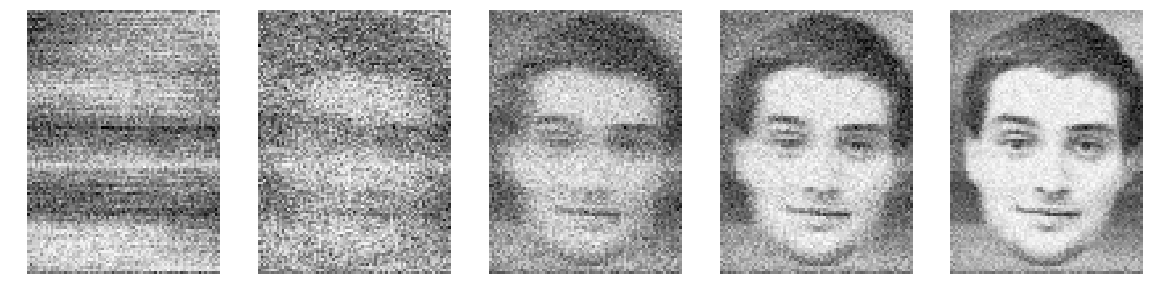
Who is the prankster?
To speed up the computation, we will perform 5 iterations over small subset of images and then gradually increase the subset.
If everything is implemented correctly, you will recognize the prankster (remember he is the one from DeepBayes team).
Run EM-algorithm:
1
2
3
4
5
6
7
defshow(F, i=1, n=1): """ shows face F at subplot i out of n """ plt.subplot(1, n, i) plt.imshow(F, cmap="Greys_r") plt.axis("off")
If you have some time left, you can implement simplified version of EM-algorithm called hard-EM. In hard-EM, instead of finding posterior distribution $p(d_k|X_k, F, B, s, A)$ at E-step, we just remember its argmax $\tilde d_k$ for each image $k$. Thus, the distribution q is replaced with a singular distribution:
This modification simplifies formulas for $\mathcal{L}$ and M-step and speeds their computation up. However, the convergence of hard-EM is usually slow.
If you implement hard-EM, add binary flag hard_EM to the parameters of the following functions:
calculate_lower_bound
run_e_step
run_m_step
run_EM
After implementation, compare overall computation time for EM and hard-EM till recognizable F.