Note for Inference Algorithms in Probabilistic ML

Record the principles and derivations of algorithms used for inferring unknown variables in probabilistic machine learning, such as Variational Inference, Expectation Maximization, and Markov Chain Monte Carlo. Many contents and derivations, as well as images, come from the online course and lecture notes of Professor Xu Yida at the University of Technology Sydney. Professor Xu's series of videos on non-parametric Bayesian methods are very good, and you can find the videos by searching his name on Bilibili or Youku. The address of Professor Xu's course notes is roboticcam/machine-learning-notes. Unless otherwise specified, some screenshots and code are from Professor Xu's lecture notes. Other contents come from various books or tutorials, and the references will be indicated in the text.

iwWPun.png

切换中文

Bayesian Inference

• In Bayesian inference, it is necessary to distinguish observable quantities (data) from unknown variables (which may be statistical parameters, missing data, or latent variables)
• Statistical parameters are regarded as random variables in the Bayesian framework, and we need to make probabilistic estimates of the model's parameters. In the frequentist framework, parameters are determined and non-random quantities, mainly used for probabilistic estimates of the data
• In the frequentist framework, only the likelihood is focused on \(p(x|\theta)\) , while the Bayesian school believes that the parameters \(\theta\) should be treated as variables, making prior assumptions about the parameters \(p(\theta)\) before observing the data
• Posterior proportionality to the product of likelihood and prior, representing the parameter probability distribution we obtain after adjusting the prior for the observed data
• In the Bayesian framework, we are more concerned with precision, which is the reciprocal of variance, for example, in the posterior of a normal distribution, precision is the sum of the precision of the prior and the data
• The posterior is actually a balance between the maximum likelihood estimation and the prior
• As the amount of data increases, the posterior gradually ceases to depend on the prior
• Many times, we do not have prior knowledge, in which case a flat, dispersed distribution is generally used as the prior distribution, such as a uniform distribution with a wide range or a normal distribution with a large variance
• Sometimes we do not need to know the entire posterior distribution but only make some point estimates or interval estimates

Markov Chain Monte Carlo

• MCMC, the first MC stands for how to sample so that the sampling points satisfy the distribution, and the second MC stands for using random sampling to estimate the parameters of the distribution
• Maximum likelihood estimation and the EM algorithm are both point estimations, while MCMC finds the complete posterior distribution through sampling
• Monte Carlo simple sampling is known for its distribution, but it is not possible to directly calculate certain statistics of functions on this distribution. Therefore, statistics are indirectly calculated by generating samples through random sampling of this distribution and then using the samples to compute the statistics
• Monte Carlo inference involves an unknown distribution and known samples (data), where the distribution is inferred from the samples (question mark pending determination)

Sampling

• It is difficult (or the distribution is unknown) to derive some statistical quantities directly through the distribution function; we can obtain the statistical quantities by generating a series of samples that conform to this distribution and calculating the statistical quantities through sample statistics, i.e., by random sampling

• In parameter inference, we can randomly sample a series of samples from the posterior distribution that satisfies the parameters, thereby estimating the parameters based on the samples

• The simplest sampling: inverse sampling from the cumulative distribution function, which is first performing a uniform distribution sampling from [0,1], and then using this value as the output of the cdf function; the sampling value is the input to the cdf:

  \[ u = U(0,1) \\ x= cdf ^{-1} (u) \\ \]

Refuse Sampling

• Not all cumulative distribution functions of distributions are easy to invert. Another sampling method is called rejection sampling.

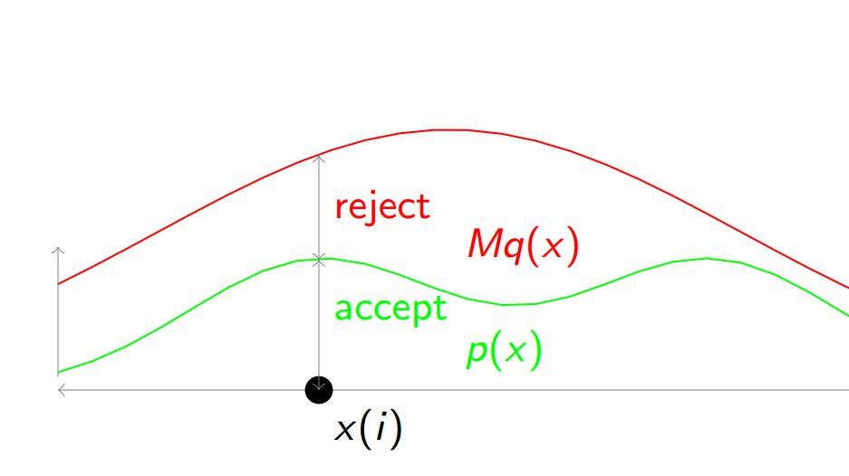
• For a probability density function, we cannot sample it directly, so we construct a distribution that is everywhere greater than the probability density function, surrounding this function, as shown in the figure where the red line encloses the green line

• We calculate the distance of each point to the red line and the green line, dividing it into acceptance and rejection regions. Thus, we first sample from the red distribution to obtain samples, and then perform a [0,1] uniform distribution sampling. If the sample falls within the acceptance region, it is accepted; otherwise, it is rejected

• 显然红色分布处处比绿色大是不可能的，积分不为 1，因此需要按比例放缩一下，乘以一个系数 M，算法如下：

  i=0
  while i!= N
  x(i)~q(x) and u~U(0,1)
  if u< p(x(i))/Mq(x(i)) then
     accept x(i)
     i=i+1
  else
     reject x(i)
  end
  end

• rejection sampling efficiency is too low because if the red distribution is not chosen well, and it cannot tightly enclose the green distribution, the acceptance rate is too low, and most samples will be rejected.

Adaptive Rejection Sampling

• When the distribution is log-concave, we can effectively construct the envelope of the green distribution, which means the red distribution is closer to the green distribution and has a higher acceptance rate
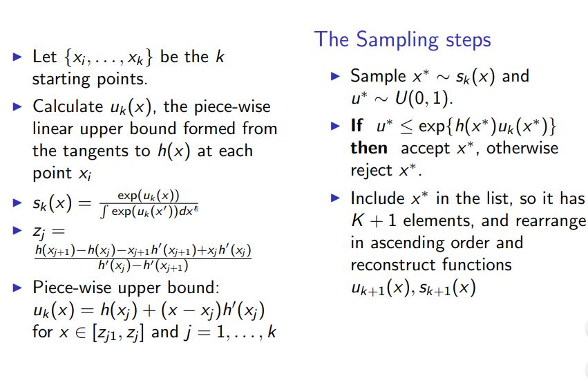
• The basic idea is to divide the green distribution to be sampled into k regions, with the leftmost point in each region serving as the starting point. If the green distribution at the starting point in each region can be enveloped by its tangent line, we can then use the tangent lines on these k regions to form the red region
• However, this requires that the original distribution be concave in each region, but for example, the probability density function of the Gaussian distribution is not a concave function; however, the Gaussian distribution becomes concave after taking the logarithm, which is what is called log-concave. Therefore, we first take the logarithm, draw the tangent, and then calculate the exponential to return to the original distribution, obtaining the k-segment tangents of the original distribution.

Importance Sampling

• The sampling algorithm mentioned above samples from a simple distribution (proposed distribution), calculates the acceptance rate for each sample through the relationship between the simple distribution and the complex distribution, and rejects some samples to ensure that the remaining samples satisfy the complex distribution

• The idea of importance sampling is to weight the sample points rather than simply rejecting or accepting them, thus fully utilizing each sample point.

• For example, we hope to obtain the expected value of a distribution through sampling

  \[ E_{p(x)}(f(x)) = \int _x f(x)p(x)dx \\ E_{p(x)}(f(x)) = \int _x f(x) \frac{p(x)}{q(x)} q(x) dx \\ E_{p(x)}(f(x)) = \int _x g(x)q(x)dx \\ \]

• p(x) is difficult to sample, so we convert it to sampling from q(x). Here, \(\frac{p(x)}{q(x)}\) represents the importance weight.

• We thus eliminate the restriction that the red distribution must envelop the green distribution, as long as we calculate the importance weights and perform importance weighting on the sampled points, we can obtain some statistical quantities under the green distribution.

Markov Monte Carlo and Metropolis-Hastings algorithms

• MCMC is another sampling method, where the sample sequence is regarded as a Markov chain, and the samples sampled by MCMC are not independent; the probability distribution of the next sample is related to the previous sample

• Different from the concepts of general sampling acceptance or rejection, MCMC calculates the probability distribution of the next sample's position under the premise of the current sample after each sample, which is the key transition probability.

• After sampling a sample, we draw the next one according to the transition probability, obtaining a series of samples that conform to the given distribution. It is evident that the transition probability needs to be related to the given distribution. We utilize the convergence of the Markov chain, hoping that the distribution after convergence, denoted as \(\pi\) , is the given distribution, assuming the transition probability is denoted as \(k(x^{'} | x)\) , from sample \(x\) to sample \(x^{'}\) .

• In the Markov chain, there is the following Chapman-Kolmogorov equation:

  \[ \pi _t (x^{'}) = \int _x \pi _{t-1}(x) k(x^{'} | x) dx \]

• The significance of this formula is self-evident. We hope to achieve the convergence of Markov chains. After convergence, regardless of how the transition is made, the sequence of samples obtained should satisfy the same given distribution, then the requirement is:

  \[ \pi _t (x) = \pi _{t-1} (x) \]

• Actual use relies on another important formula, known as the detailed balance condition:

  \[ \pi (x) k(x^{'} | x) = \pi (x^{'}) k(x | x^{'}) \]

• From detailed balance, it can be deduced that the Chapman-Kologronvo equation holds, but the converse is not necessarily true.

• When the detailed balance condition is satisfied, the Markov chain is convergent

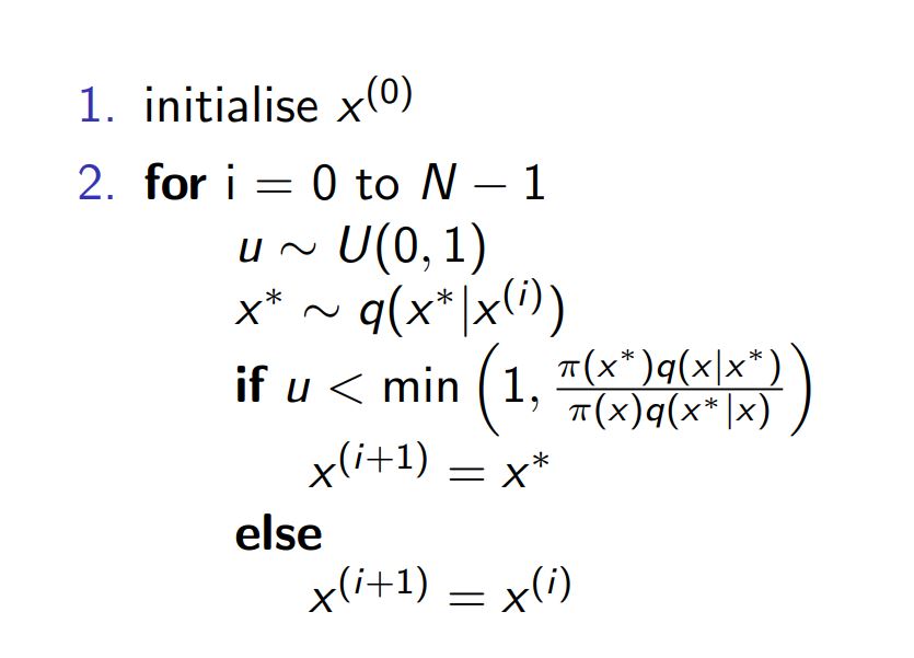
• In the LDA blog, mh and Gibbs are introduced, and Metropolis-Hasting is the result of the basic MCMC where the acceptance rate on one side is raised to 1:

• In the mh, we did not alter the transition matrix to adapt to the given distribution, but instead used the given distribution to correct the transition matrix, thus, the transition matrix is one that we ourselves designed. Generally, the transition matrix (proposal distribution) is designed as a Gaussian distribution centered around the current state. For this Gaussian distribution, when the variance is small, the probability is concentrated around the current sampling point, so the position transferred to the next sampling point is unlikely to change much, resulting in a high acceptance rate (since the current sampling point is the one that passed the acceptance, it is likely to be in a position with a high acceptance rate). However, this will cause the random walk to be slow; if the variance is large, it will wander everywhere, and the acceptance rate will decrease.

• Despite one side's sample acceptance rate reaching 1, there is always one side below 1. If it is rejected, the MCMC will repeat sampling at the same location once and then continue.

• And Gibbs raised both acceptance rates to 1, which shows that Gibbs is a special case of MCMC. MCMC does not modify the transition probability but adds the acceptance rate, linking the original transition probability with the distribution to be sampled. However, it is obvious that if we ourselves choose the transition probability and make it more closely related to the original distribution, the effect will be better, and Gibbs follows this approach.

Hybrid Metropolis-Hasting

• To be supplemented

Gibbs Sampling

• A motivation for Gibbs sampling: It is difficult to sample directly from the joint distribution of multiple parameters, but if other parameters are fixed as conditions, sampling from the conditional distribution of just one parameter becomes much simpler, and it can be proven that the samples obtained after convergence satisfy the joint distribution

• Firstly, let's consider why the Gibbs sampling process does not change the joint probability distribution through iterative conditional sampling. Firstly, when excluding the i-th parameter to calculate the conditional probability, the marginal distribution of the excluded n-1 variables is the same as the marginal distribution of the true joint probability distribution for these n-1 variables, because their values have not changed; the condition on which the conditional probability is based is unchanged compared to the true distribution, so the conditional probability distribution is also unchanged. Both the marginal distribution and the conditional probability distribution are unchanged (true), so the joint distribution obtained by multiplying them is naturally unchanged, and therefore, in each iteration step, sampling is done according to the true distribution and the iteration does not change this distribution.

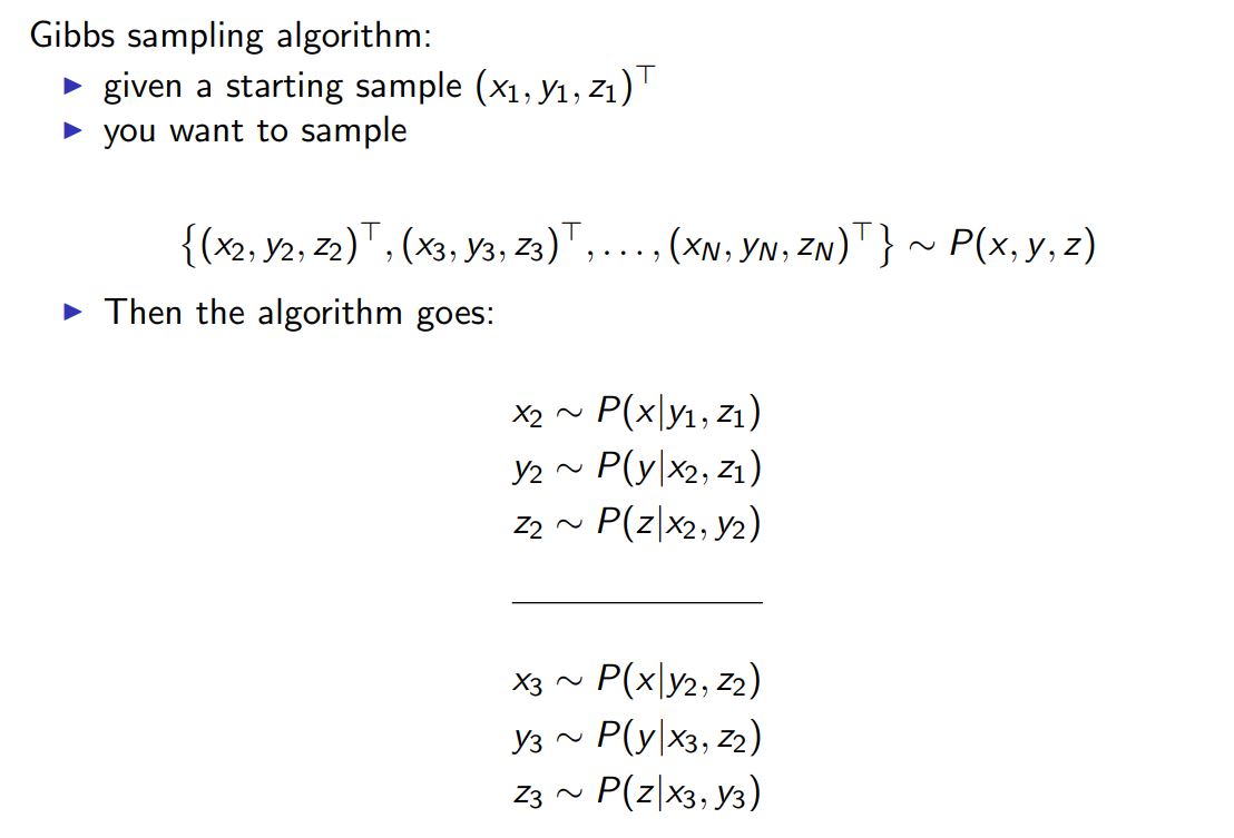
• Gibbs sampling is a coordinate descent method similar to variational inference, updating one component of the sample at a time, based on the conditional probability of the current updating component's dimension given the other components:

• Industrial applications of Gibbs sampling are widespread due to its speed. In fact, such an iterative algorithm cannot be parallelized, but the collapsed Gibbs sampling can parallelize the iteration. The principle is to treat several components as a whole, collapsing them into one component. When other components are updated using this set of components, they are considered independent (there is some doubt; another way to describe collapse is to ignore some conditional variables. Basic Gibbs sampling is essentially collapsed Gibbs sampling, and the approach of treating several components as a whole is blocked Gibbs sampling):

  u~p(u|x,y,z)
  x,y,z~p(x,y,z|u)
  =p(x|u)p(y|u)p(z|u)

• The three conditional probabilities concerning x, y, and z can be computed in parallel.

• Now we prove that Gibbs is a special case of Metropolis-Hastings with an acceptance rate of 1, let's first look at the acceptance rate of Metropolis-Hastings

  \[ \alpha = min(1,\frac{\pi (x^{'}),q(x| x^{'})}{\pi (x) q(x^{'} | x)}) \]

• In Gibbs

  \[ q(x|x^{'})=\pi (x_i | x_{¬i}^{'}) \\ q(x^{'}|x)=\pi (x_i ^{'} | x_{¬i}) \\ \]

• And in fact, from \(x_{¬i}\) to \(x_{¬i}^{'}\) , only the ith component changes, with the other components remaining unchanged, therefore

  \[ x_{¬i}^{'}=x_{¬i} \]

• Next, let's examine Gibbs' acceptance rate

  \[ \alpha _{gibbs} = min(1,\frac{\pi (x^{'}) \pi (x_i | x_{¬i}^{'})}{\pi (x) (x_i ^{'} | x_{¬i})}) \\ \]

  \[ = min(1,\frac{\pi (x^{'}) \pi (x_i | x_{¬i})}{\pi (x) (x_i ^{'} | x_{¬i})}) \\ \]

  \[ = min(1,\frac{\pi (x^{'} | x_{¬i}^{'}) \pi( x_{¬i}^{'}) \pi (x_i | x_{¬i})}{\pi (x_i | x_{¬i}) \pi( x_{¬i}) (x_i ^{'} | x_{¬i})}) \\ \]

  \[ = min(1,\frac{\pi (x^{'} | x_{¬i}) \pi( x_{¬i}) \pi (x_i | x_{¬i})}{\pi (x_i | x_{¬i}) \pi( x_{¬i}) (x_i ^{'} | x_{¬i})}) \\ \]

  \[ = min(1,1) \\ \]

  \[ = 1 \\ \]

Expectation Maximization

Update

• deep|bayes2018 mentions using stochastic gradient descent for the M-step in EM, as it is stochastic, the E-step only targets a portion of the data, reducing overhead, and enabling inference of latent variable models on large-scale datasets. At the time, it was applied to word2vec, adding a qualitative latent variable for each word to indicate one of its multiple meanings, aiming to resolve ambiguity issues, and even parameterize the number of word meanings using the Chinese restaurant process. Will look at it in detail when I have time.

Formula

• For simple distributions, we want to perform parameter inference, which only requires maximum likelihood estimation, first calculating the log-likelihood:

\[ \theta=\mathop{argmax}_{\theta} L(X | \theta) \\ =\mathop{argmax}_{\theta} \log \prod p(x_i | \theta) \\ =\mathop{argmax}_{\theta} \sum \log p(x_i | \theta) \\ \]

• Afterward, differentiate the log-likelihood to calculate the extrema; however, for complex distributions, it may not be convenient to differentiate

• We can use the EM algorithm to iteratively solve this. The EM algorithm considers the latent variables in the probabilistic generative model and assigns probabilities to them, updating their probability distribution and the parameter \(\theta\) simultaneously with each iteration. It can be proven that after each iteration, the obtained \(\theta\) will increase the log-likelihood.

• Each iteration is divided into two parts, E and M, which correspond to seeking the expectation and maximization

  • The expectation is the expectation of \(\log p(x,z|\theta)\) over the distribution \(p(z|x,\theta ^{(t)})\) , where \(\theta ^{(t)}\) is the parameter calculated at the t-th iteration
  • Maximization, that is, seeking the \(\theta\) that maximizes this expectation, as the result of the parameter update in this iteration

• The formula for the EM algorithm is obtained when combined:

  \[ \theta ^{(t+1)} = \mathop{argmax} _{\theta} \int p(z|x,\theta ^{(t)}) \log p(x,z|\theta) dz \]

  Why Effective

• That is to prove, the maximum likelihood will increase after each iteration

• To prove:

  \[ \log p(x|\theta ^{(t+1)}) \geq \log p(x|\theta ^{(t)}) \]

• Reformulate the log-likelihood

  \[ \log p(x|\theta) = \log p(x,z|\theta) - \log p(z|x,\theta) \\ \]

• Both sides of the distribution \(p(z|x,\theta ^{(t)})\) calculate the expectation, noting that the left side of the equation is independent of z, therefore, after calculating the expectation, it remains unchanged:

  \[ \log p(x|\theta) = \int _z \log p(x,z|\theta) p(z|x,\theta ^{(t)}) dz - \int _z \log p(z|x,\theta) p(z|x,\theta ^{(t)}) dz \\ =Q(\theta,\theta ^{(t)})-H(\theta,\theta ^{(t)}) \\ \]

• The Q part is the E part of the EM algorithm, note that here \(\theta\) is a variable, \(\theta ^{(t)}\) is a constant

• After the iteration, due to the role of the M part in the EM algorithm, the Q part must have increased (greater than or equal to), then what will the new \(\theta\) after this iteration that makes the Q part increase change when substituted into the H part?

• We first calculate, assuming that the \(\theta\) of section H remains unchanged, directly using the previous \(\theta ^{(t)}\) to input, that is, \(H(\theta ^{(t)},\theta ^{(t)})\)

  \[ H(\theta ^{(t)},\theta ^{(t)})-H(\theta,\theta ^{(t)})= \\ \]

  \[ \int _z \log p(z|x,\theta ^{(t)}) p(z|x,\theta ^{(t)}) dz - \int _z \log p(z|x,\theta) p(z|x,\theta ^{(t)}) dz \\ \]

  \[ = \int _z \log (\frac {p(z|x,\theta ^{(t)})} {p(z|x,\theta)} ) p(z|x,\theta ^{(t)}) dz \\ \]

  \[ = - \int _z \log (\frac {p(z|x,\theta)} {p(z|x,\theta ^{(t)})} ) p(z|x,\theta ^{(t)}) dz \\ \]

  \[ \geq - \log \int _z (\frac {p(z|x,\theta)} {p(z|x,\theta ^{(t)})} ) p(z|x,\theta ^{(t)}) dz \\ \]

  \[ = - \log 1 \\ \]

  \[ = 0 \\ \]

• The inequality in question utilizes the Jensen inequality. That is, directly using the previous \(\theta ^{(t)}\) as \(\theta\) to substitute into H is the maximum value of H! Then, regardless of how much \(\theta ^{(t+1)}\) is obtained from the new argmax Q part, substituting it into H will cause the H part to decrease (less than or equal to) ! The numerator becomes larger, and the denominator smaller, so the result is that the log-likelihood is definitely larger, which proves the effectiveness of the EM algorithm.

Understanding from the perspective of the Evidence Lower Bound (ELBO)

• We can also derive the formula for the EM algorithm from the perspective of ELBO (Evidence Lower Bound)

• In the previous rewriting of the log-likelihood, we obtained two expressions \(p(x,z|\theta)\) and \(p(z|x,\theta)\) . We introduce a distribution \(q(z)\) of latent variables, and by computing the KL divergence between these two expressions and \(q(z)\) , we can prove that the log-likelihood is the difference between these two KL divergences:

  \[ KL(q(z)||p(z|x,\theta)) = \int q(z) [\log q(z) - \log p(z|x,\theta)] dz \\ \]

  \[ = \int q(z) [\log q(z) - \log p(x|z,\theta) - \log (z|\theta) + \log p(x|\theta)] dz \\ \]

  \[ = \int q(z) [\log q(z) - \log p(x|z,\theta) - \log (z|\theta)] dz + \log p(x|\theta) \\ \]

  \[ = \int q(z) [\log q(z) - \log p(x,z|\theta)] dz + \log p(x|\theta) \\ \]

  \[ = KL(q(z)||p(x,z|\theta)) + \log p(x|\theta) \\ \]

• That is to say

  \[ \log p(x|\theta) = - KL(q(z)||p(x,z|\theta)) + KL(q(z)||p(z|x,\theta)) \]

• ELBO is the evidence lower bound, because of \(KL(q(z)||p(z|x,\theta)) \geq 0\) , thus ELBO is a lower bound for the log-likelihood. We can maximize this lower bound to maximize the log-likelihood.

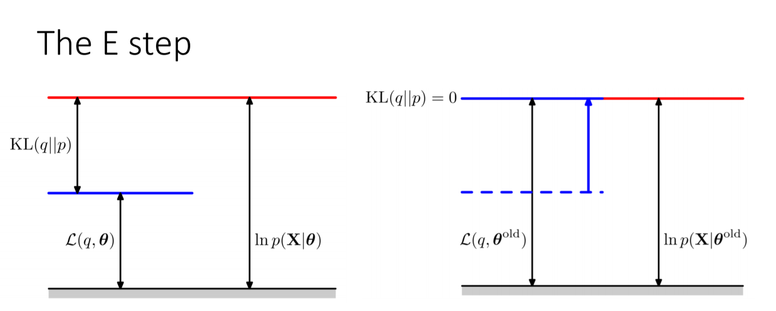
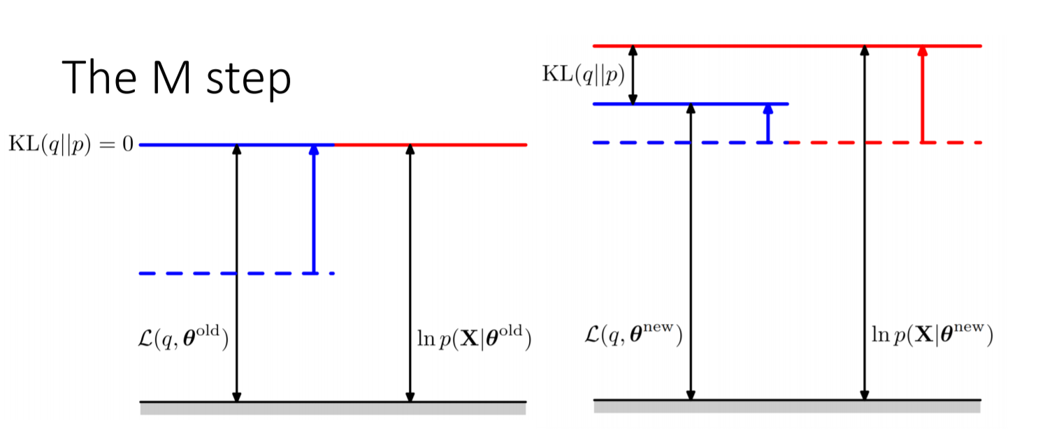
• It can be seen that the ELBO has two parameters, \(q\) and \(\theta\) . First, we fix \(\theta ^{(t-1)}\) , and find the \(q^{(t)}\) that maximizes the ELBO, which is actually the E-step of the EM algorithm. Next, we fix \(q^{(t)}\) , and find the \(\theta ^{(t)}\) that maximizes the ELBO, which corresponds to the M-step of the EM algorithm

• We substitute \(\theta = \theta ^{(t-1)}\) into the ELBO expression:

  \[ ELBO=\log p(x|\theta ^{(t-1)}) - KL(q(z)||p(z|x,\theta ^{(t-1)})) \]

• What value of q maximizes the ELBO? It is obvious that when the KL divergence is 0, the ELBO reaches its maximum value, which is when the lower bound reaches the logarithmic likelihood itself, at which point \(q(z)=p(z|x,\theta ^{(t-1)})\) , next we fix \(q\) , and seek the value of \(\theta\) that maximizes the ELBO, first rewriting the definition of ELBO:

  \[ ELBO = - KL(q(z)||p(x,z|\theta)) \\ \]

  \[ = \int q^{(t)}(z) [ \log p(x,z|\theta) - \log q^{(t)}(z)] dz \\ \]

  \[ = - \int q^{(t)}(z) \log p(x,z|\theta) - q^{(t)}(z) \log q^{(t)}(z) dz \\ \]

• The second item is unrelated to \(\theta\) , therefore:

  \[ \theta ^{(t)} = \mathop{argmax} _{\theta} \int q^{(t)}(z) \log p(x,z|\theta) dz \\ \]

• Substitute the \(q(z)=p(z|x,\theta ^{(t-1)})\) obtained in the previous step, and we get

  \[ \theta ^{(t)} = \mathop{argmax} _{\theta} \int \log p(x,z|\theta)p(z|x,\theta ^{(t-1)}) dz \]

• Similarly, the iterative formula of the EM algorithm is obtained

• The following two figures are extracted from Christopher M. Bishop's Pattern Recognition and Machine Learning, illustrating what the E-step and M-step actually do: The E-step raises the lower bound ELBO to the log-likelihood, but at this point only the latent variables are updated, so the log-likelihood does not change. When the updated latent variables are used to update the parameters \(\theta\) , i.e., after the M-step is executed, we continue to obtain a higher ELBO and its corresponding log-likelihood. At this time, q does not change, but p changes, so KL is not 0, and the log-likelihood must be greater than the ELBO, i.e., it will increase. Intuitively, we increase the ELBO in both the E and M steps; the E-step first raises the ELBO to the log-likelihood in one go, and then the M-step can still increase the ELBO, but the log-likelihood will definitely be greater than or equal to (in fact, greater than) the ELBO at the M-step, so the log-likelihood is "pushed up" by the ELBO increased by the M-step.

• The remaining issue is how to select z and q; in the mixed model, z can be introduced as an indicator function, while the other probability models containing latent variables can directly introduce the latent variables during design

From the perspective of assuming latent variables to be observable

• This understanding comes from the tutorial by Chuong B Do & Serafim Batzoglou: What is the Expectation Maximization Algorithm?
• EM is used for inference in probabilistic models with unobserved latent variables. In fact, if we make the latent variables observable from unobserved, and perform maximum likelihood estimation for each possible value of the latent variables, we can still obtain results, but the time cost is quite high.
• EM then improves this naive algorithm. One understanding of the EM algorithm is: The EM algorithm first guesses a probability distribution of the hidden variables in each iteration, creates a weighted training set considering all possible values of the hidden variables, and then performs a modified version of maximum likelihood estimation on it.
• Guessing the probability distribution of a hidden variable is the E-step, but we do not need to know the specific probability distribution; we only need to calculate the expectation of the sufficient statistic on this distribution.
• The EM algorithm is a natural generalization of maximum likelihood estimation to data containing hidden variables (or data containing partially unobserved samples).

From the perspective of missing values in the latent variables

• How are missing values generally handled? Replaced with random values, mean values, 0 values, cluster center values, etc
• EM is equivalent to replacing missing values with the mean, i.e., the latent variable, but it utilizes more information: this mean is obtained by taking the expectation over the known distribution of x
• The EM iteration involves repeatedly processing missing values (latent variables), then adjusting the distribution of x based on the complete data, and finally treating the latent variables as missing values for adjustment

EM algorithm and K-means

• K-means is a Hard-EM algorithm that, like the EM algorithm, makes assumptions about various possible latent variables (the class to which the sample belongs), but it does not calculate probabilities and expectations on the class level. Instead, it is more rigid, specifying only one class as the sample's class, with a probability of 1 for this class and 0 for all others.

Benefits of Introducing Latent Variables

• In fact, it should be said the other way around: many times, we design latent variables based on logic and then use the EM algorithm to infer the latent variables, rather than deliberately designing latent variables to simplify computation.

• For GMM, one advantage of introducing latent variables is that it simplifies the computation of maximum likelihood estimation (of course, this is under the assumption that we know the latent variables), by exchanging the logarithm with the summation operation, referring to the blog of the great pluskid: On Clustering (Extra Chapter): Expectation Maximization

• Before introducing latent variables as indicator functions for GMM, the maximum likelihood estimation is:

  \[ \sum _{i=1}^N \log (\sum _{k=1}^K \pi _k N(x_i | \mu _k , \Sigma _k)) \]

• After introducing latent variables, the indicator function corresponding to the ith sample \(x_i\) is \(z_i\) , which is a k-dimensional one-hot vector representing which of the k Gaussian models the ith sample belongs to. If it belongs to the mth model, then \(z_i^m\) equals 1, and the rest are 0. Now, the maximum likelihood estimation is:

  \[ \log \prod _{i=1}^N p(x_i,z_i) \\ \]

  \[ = \log \prod _{i=1}^N p(z_i) \prod _{k=1}^K N(x_i | \mu _k , \Sigma _k)^{z_i^k} \\ \]

  \[ = \log \prod _{i=1}^N \prod _{k=1}^K \pi _k ^{z_i^k} \prod _{k=1}^K N(x_i | \mu _k , \Sigma _k)^{z_i^k} \\ \]

  \[ = \log \prod _{i=1}^N \prod _{k=1}^K ( \pi _k N(x_i | \mu _k , \Sigma _k)) ^{z_i^k} \\ \]

  \[ = \sum _{i=1}^N \sum _{k=1}^K z_i^k(\log \pi _k + \log N(x_i | \mu _k , \Sigma _k)) \\ \]

Application of Monte Carlo Method in the EM Algorithm

• When the E-step cannot parse the computation, the integral of the M-step can be approximated using Monte Carlo methods:

  \[ \theta ^{(t+1)} = \mathop{argmax} _{\theta} \int p(z|x,\theta ^{(t)}) \log p(x,z|\theta) dz \]

• We sample a finite number of \(Z^l\) based on the posterior estimate \(p(z|x,\theta ^{(t)})\) of the latent variables obtained now, and then substitute these \(Z^l\) into \(\log p(x,z|\theta)\) to approximate the integral:

  \[ \theta ^{(t+1)} = \mathop{argmax} _{\theta} \approx \frac 1L \sum_{l=1}^L \log p(x,Z^l|\theta) \]

• An extreme example of the Monte Carlo EM algorithm is the random EM algorithm, which is equivalent to sampling only one sample point in the E-step at each iteration. In the solution of mixed models, the latent variables act as indicator functions, and sampling only one latent variable implies hard assignment, with each sample point assigned to a component with a probability of 1.

• Monte Carlo EM algorithm extended to the Bayesian framework results in the IP algorithm

  • I steps:

    \[ p(Z|X)=\int p(Z | \theta ,X)p(\theta | X)d\theta \]

    Sample from \(p(\theta | X)\) , then substitute into it, and subsequently sample from \(p(Z | \theta ^l ,X)\) into \(Z^l\) .

  • P-step: Sampling from the I-step obtained \(Z^l\) for estimating the posterior parameters:

    \[ p(\theta | X) = \int p(\theta | Z,X)p(Z|X) dZ \\ \approx \frac 1L \sum _{l=1}^L p(\theta | Z^l,X) \\ \]

Generalized EM Algorithm

• Will not chicken out

Wake-Sleep algorithm

• Pigeon Ethics Philosophy

Generalized EM Algorithm and Gibbs Sampling

• When you think I won't chicken out and I do, it's also a form of not chickening out

Variational Inference

ELBO

• Next, we introduce variational inference, and it can be seen that the EM algorithm can be generalized to variational inference

• Reintroducing the relationship between ELBO and log-likelihood:

  \[ \log p(x) = \log p(x,z) - \log p(z|x) \\ = \log \frac{p(x,z)}{q(z)} - \log \frac{p(z|x)}{q(z)} \\ = \log p(x,z) - \log q(z) - \log \frac{p(z|x)}{q(z)} \\ \]

• Seek the expectation of the hidden distribution \(q(z)\) on both sides

  \[ \log p(x) = \\ [ \int _z q(z) \log p(x,z)dz - \int _z q(z) \log q(z)dz ] + [- \int _z \log \frac{p(z|x)}{q(z)} q(z) dz ]\\ = ELBO+KL(q||p(z|x)) \\ \]

• We hope to infer the posterior distribution of the latent variable \(z\) , for this purpose, we introduce a distribution \(q(z)\) to approximate this posterior. Under the premise of the current observations, i.e., the log-likelihood, the approximation of the posterior is equivalent to minimizing the KL divergence between \(q(z)\) and \(p(z|x)\) . From the above formula, it can be seen that when the ELBO is maximized, the KL divergence is minimized.

• Next is the discussion on how to maximize the ELBO

Variational inference on arbitrary distributions

• For any distribution, update one component of the latent variable at a time, such as the jth component

• Ourself-selected \(q(z)\) is of course simpler than the approximate distribution; here, it is assumed that the distribution is independent, and the latent variable is \(M\) -dimensional:

  \[ q(z)=\prod _{i=1}^M q_i(z_i) \]

• Therefore, the ELBO can be expressed in two parts

  \[ ELBO=\int \prod q_i(z_i) \log p(x,z) dz - \int \prod q_j(z_j) \sum \log q_j(z_j) dz \\ =part1-part2 \\ \]

• The part1 can be expressed in the form of multiple integrals over the various dimensions of the latent variables, and we select the jth dimension to rewrite it as

  \[ part1=\int \prod q_i(z_i) \log p(x,z) dz \\ \]

  \[ = \int _{z_1} \int _{z_2} ... \int _{z_M} \prod _{i=1}^M q_i(z_i) \log p(x,z) d z_1 , d z_2 , ... ,d z_M \\ \]

  \[ = \int _{z_j} q_j(z_j) ( \int _{z_{i \neq j}} \log (p(x,z)) \prod _{z_{i \neq j}} q_i(z_i) d z_i) d z_j \\ \]

  \[ = \int _{z_j} q_j(z_j) [E_{i \neq j} [\log (p(x,z))]] d z_j \\ \]

• In this context, we define a form of pseudo-distribution, which is the pseudo-distribution of a distribution, obtained by integrating the logarithm of the distribution and then exponentiating the result:

  \[ p_j(z_j) = \int _{i \neq j} p(z_1,...,z_i) d z_1 , d z_2 ,..., d z_i \\ \]

  \[ p_j^{'}(z_j) = exp \int _{i \neq j} \log p(z_1,...,z_i) d z_1 , d z_2 ,..., d z_i \\ \]

  \[ \log p_j^{'}(z_j) = \int _{i \neq j} \log p(z_1,...,z_i) d z_1 , d z_2 ,..., d z_i \\ \]

• This part 1 can be rewritten in the form of pseudo-distribution

  \[ part1= \int _{z_j} q_j(z_j) \log p_j^{'}(x,z_j) \\ \]

• In part 2, because the components of the latent variables are independent, the sum of the function can be rewritten as the sum of the expectations of each function over the marginal distributions, in which we focus on the j-th variable, treating the rest as constants:

  \[ part2=\int \prod q_j(z_j) \sum \log q_j(z_j) dz \\ \]

  \[ = \sum ( \int q_i(z_i) \log (q_i(z_i)) d z_i ) \\ \]

  \[ = \int q_j(z_j) \log (q_j(z_j)) d z_j + const \\ \]

• Combine part 1 and part 2 to obtain the form of the ELBO for component j:

  \[ ELBO = \int _{z_j} \log \log p_j^{'}(x,z_j) - \int q_j(z_j) \log (q_j(z_j)) d z_j + const \\ \]

  \[ = \int _{z_j} q_j(z_j) \log \frac{p_j^{'}(x,z_j)}{q_j(z_j)} + const \\ \]

  \[ = - KL(p_j^{'}(x,z_j) || q_j(z_j)) + const\\ \]

• The ELBO is written as the negative KL divergence between a pseudo-distribution and an approximate distribution, maximizing the ELBO is equivalent to minimizing this KL divergence

• When is this KL divergence minimum? That is to say:

  \[ q_j(z_j) = p_j^{'}(x,z_j) \\ \log q_j(z_j) = E_{i \neq j} [\log (p(x,z))] \\ \]

• We have obtained the iterative formula for the approximate distribution of a single component of the latent variables under variational inference. When calculating the probability of the jth component, the expectation over all other components \(q_i(z_i)\) is used, and then this new probability of the jth component participates in the next iteration, calculating the probabilities of the other components.

Exponential family distribution

• Define the exponential family distribution:

  \[ p(x | \theta)=h(x) exp(\eta (\theta) \cdot T(x)-A(\theta)) \\ \]

• Amongst

  • sufficient statistics
  • \(\theta\):parameter of the family
  • \(\eta\):natural parameter
  • underlying measure
  • \(A(\theta)\) : log normalizer / partition function

• Attention: The parameter of the family and the natural parameter are both vectors. When the exponential family distribution is in the form of scalar parameters, i.e., \(\eta _i (\theta) = \theta _i\) , the exponential family distribution can be written as:

  \[ p(x | \eta)=h(x) exp(\eta (T(x) ^T \eta - A(\eta)) \]

• When we express the probability density function in the exponential family form, we have:

  \[ \eta = \mathop{argmax} _ {\eta} [\log p(X | \eta)] \\ \]

  \[ = \mathop{argmax} _ {\eta} [\log \prod p(x_i | \eta)] \\ \]

  \[ = \mathop{argmax} _ {\eta} [\log [\prod h(x_i) exp [(\sum T(x_i))^T \eta - n A(\eta)]]] \\ \]

  \[ = \mathop{argmax} _ {\eta} (\sum T(x_i))^T \eta - n A(\eta)] \\ \]

  \[ = \mathop{argmax} _ {\eta} L(\eta) \\ \]

• Continuing to seek extrema, we can obtain a very important property of the exponential family distribution regarding the log normalizer and sufficient statistics:

  \[ \frac{\partial L (\eta)}{\partial \eta} = \sum T(x_i) - n A^{'}(\eta) =0 \\ \]

  \[ A^{'}(\eta) = \sum \frac{T(x_i)}{n} \\ \]

• For example, the Gaussian distribution is written in the form of an exponential family distribution:

  \[ p(x) = exp[- \frac{1}{2 \sigma ^2}x^2 + \frac{\mu}{\sigma ^2}x - \frac{\mu ^2}{2 \sigma ^2} - \frac 12 \log(2 \pi \sigma ^2)] \\ \]

  \[ =exp ( [x \ x^2] [\frac{\mu}{\sigma ^2} \ \frac{-1}{2 \sigma ^2}] ^T - \frac{\mu ^2}{2 \sigma ^2} - \frac 12 \log(2 \pi \sigma ^2) ) \]

• Using natural parameters to replace variance and mean, expressed in the exponential family distribution form:

  \[ p(x) = exp( [x \ x^2] [ \eta _1 \ \eta _2] ^T + \frac{\eta _1 ^2}{4 \eta _2} + \frac 12 \log (-2 \eta _2 ) - \frac 12 \log (2 \pi)) \]

• Wherein:

  • \(T(x)\):\([x \ x^2]\)
  • \(\eta\):\([ \eta _1 \ \eta _2] ^T\)
  • \(-A(\eta)\):\(\frac{\eta _1 ^2}{4 \eta _2} + \frac 12 \log (-2 \eta _2 )\)

• Next, we utilize the properties of the exponential family to quickly calculate the mean and variance

  \[ A^{'}(\eta) = \sum \frac{T(x_i)}{n} \\ \]

  \[ [\frac{\partial A}{\eta _1} \ \frac{\partial A}{\eta _2}] = [\frac{- \eta _1}{2 \eta _2} \ \frac{\eta _1 ^2 }{2 \eta _2}-\frac{1}{2 \eta _2}] \\ \]

  \[ = [\frac{\sum x_i}{n} \ \frac{\sum x_i^2}{n}] \\ \]

  \[ = [\mu \ \mu ^2 + \sigma ^2] \\ \]

• Why is \(A(\eta)\) called log normalizer? Because the integral of the exponential family distribution of the probability density has:

  \[ \int _x \frac{h(x)exp(T(x)^T \eta)}{exp(A(\eta))} = 1 \\ \]

  \[ A(\eta) = \log \int _x h(x)exp(T(x)^T \eta) \\ \]

• Below discusses the conjugate relationships of exponential family distributions, assuming that both the likelihood and the prior are exponential family distributions:

  \[ p(\beta | x) ∝ p(x | \beta) p(\beta) \\ \]

  \[ ∝ h(x) exp(T(x) \beta ^T - A_l (\beta)) h(\beta) exp(T(\beta) \alpha ^T - A(\alpha)) \\ \]

• Rewritten in the form of a vector group:

  \[ T(\beta) = [\beta \ -g(\beta)] \\ \]

  \[ \alpha = [\alpha _1 \ \alpha _2] \\ \]

• In the original expression, \(\beta\) , \(h(x)\) , and \(A(\alpha)\) are all constants, which are eliminated from the proportional expression and then substituted into the vector group:

  \[ ∝ h(\beta) exp(T(x) \beta - A_l(\beta) + \alpha _1 \beta - \alpha _2 g(\beta)) \\ \]

• We note that if we let \(-g(\beta)=-A_l (\beta)\) , the original expression can be written as:

  \[ ∝ h(\beta) exp((T(x)+\alpha _1)\beta - (1+\alpha _2) A_l (\beta)) \\ \]

  \[ ∝ h(\beta) exp(\alpha _1 ^{'} \beta - \alpha _2 ^{'} A_l (\beta)) \\ \]

• The prior and posterior forms are consistent, that is, conjugate

• We thus write down the likelihood and prior in a unified form

  \[ p(\beta | x, \alpha) ∝ p(x | \beta) p(\beta | \alpha) \\ \]

  \[ ∝ h(x)exp[T(x)^T\beta - A_l(\beta)] h(\beta) exp[T(\beta)^T\alpha - A_l(\alpha)] \\ \]

• Here we can calculate the derivative of the log normalizer with respect to the parameters, note that this is a calculated result, different from the properties of the log normalizer and sufficient statistics obtained from the maximum likelihood estimation of the exponential family distribution

  \[ \frac{\partial A_l(\beta)}{\partial \beta}=\int _x T(x) p(x | \beta)dx \\ \]

  \[ = E_{p(x|\beta)} [T(x)] \\ \]

• The above equation can be proven by integrating over the exponential family distribution with the integral equal to 1, and taking the derivative with respect to \(\beta\) yields 0, transforming this equation to prove it.

Variational Inference under Exponential Family Distributions

• Next, we will express the parameter posterior in the ELBO in the form of an exponential family distribution, and it can be seen that the final iteration formula is quite concise

• We assume that there are two parameters to be optimized, x and z, and we use \(\lambda\) and \(\phi\) to approximate \(\eta(z,x)\) and \(\eta(\beta ,x)\) . The goal remains to maximize the ELBO, at which point the adjusted parameter is \(q(\lambda , \phi)\) , which is actually \(\lambda\) and \(\phi\)

• We adopt a method of fixing one parameter and optimizing another, iteratively making the ELBO larger

• First, we rewrite the ELBO, noting \(q(z,\beta)=q(z)q(\beta)\)

  \[ ELBO=E_{q(z,\beta)}[\log p(x,z,\beta)] - E_{q(z,\beta)}[\log p(z,\beta)] \\ \]

  \[ = E_{q(z,\beta)}[\log p(\beta | x,z) + \log p(z | x) + \log p(x)] - E_{q(z,\beta)}[\log q(\beta)] - E_{q(z,\beta)}[\log q(z)] \\ \]

• The posterior is distributed in the exponential family, and the q-distribution is approximated using simple parameters \(\lambda\) and \(\phi\)

  \[ p(\beta | x,z) = h(\beta) exp [ T(\beta) ^T \eta (z,x) - A_g (\eta(z,x))] \\ \]

  \[ \approx q(\beta | \lambda) \\ \]

  \[ = h(\beta) exp [ T(\beta) ^T \eta (\lambda - A_g (\eta(\lambda))] \\ \]

  \[ p(z | x,\beta) = h(z) exp [ T(z) ^T \eta (\beta,x) - A_l (\eta(\beta,x))] \\ \]

  \[ \approx q(\beta | \phi) \\ \]

  \[ = h(z) exp [ T(z) ^T \eta (\phi - A_l (\eta(\phi))] \\ \]

• Now we fix \(\phi\) , optimize \(\lambda\) , and remove irrelevant constants from the ELBO, yielding:

  \[ ELBO_{\lambda} = E_{q(z,\beta)}[\log p(\beta | x,z)] - E_{q(z,\beta)}[\log q(\beta)] \\ \]

• Substitute the exponential family distribution, eliminate the irrelevant constant \(- E_{q(z)}[A_g(\eta(x,z))]\) , and simplify to obtain:

  \[ ELBO_{\lambda} = E_{q(\beta)}[T(\beta)^T] E_{q(z)}[\eta(z,x)] -E_{q(\beta)} [T(\beta)^T \lambda] + A_g(\lambda) \]

• Using the conclusions from the previous log normalizer regarding parameter differentiation, we have:

  \[ ELBO_{\lambda} = A_g^{'}(\lambda)^T[E_{q(z)}[\eta(z,x)]] - \lambda A_g^{'}(\lambda) ^T + A_g (\lambda) \]

• Differentiate the above equation, set it to 0, and we have:

  \[ A_g^{''}(\lambda)^T[E_{q(z)}[\eta(z,x)]] - A_g^{'}(\lambda)-\lambda A_g^{''}(\lambda) ^T + A_g^{} (\lambda) = 0 \\ \lambda = E_{q(z)}[\eta(z,x)] \\ \]

• We have obtained the iterative \(\lambda\) ! Similarly, we can obtain:

  \[ \phi = E_{q(\beta)}[\eta(\beta,x)] \\ \]

• Should be written as:

  \[ \lambda = E_{q(z | \phi)}[\eta(z,x)] \\ \phi = E_{q(\beta | \lambda)}[\eta(\beta,x)] \\ \]

• The variable update paths for these two iterative processes are:

  \[ \lambda \rightarrow q(\beta | \lambda) \rightarrow \phi \rightarrow q(z | \phi) \rightarrow \lambda \]

Bayesian Inference

• 在贝叶斯推断中，需要区别可观察量（数据）和未知变量（可能是统计参数、缺失数据、隐变量）
• 统计参数在贝叶斯框架中被看成是随机变量，我们需要对模型的参数进行概率估计，而在频率学派的框架下，参数是确定的非随机的量，主要针对数据做概率估计
• 在频率学派框架中只关注似然\(p(x|\theta)\)，而贝叶斯学派认为应将参数\(\theta\)作为变量，在观察到数据之前，对参数做出先验假设\(p(\theta)\)
• 后验正比与似然乘以先验，代表观察到数据后我们对参数先验调整，得到的参数概率分布
• 在贝叶斯框架中我们更关注精确度，它是方差的倒数，例如在正态分布的后验中，精确度是先验和数据的精确度之和
• 后验实际上是在最大似然估计和先验之间权衡
• 当数据非常多时，后验渐渐不再依赖于先验
• 很多时候我们并没有先验知识，这时一般采用平坦的、分散的分布作为先验分布，例如范围很大的均匀分布，或者方差很大的正态分布
• 有时我们并不需要知道整个后验分布，而仅仅做点估计或者区间估计

Markov Chain Monte Carlo

• MCMC，前一个MC代表如何采样，使得采样点满足分布，后一个MC代表用随机采样来估计分布的参数
• 最大似然估计和EM算法都是点估计，而MCMC是通过采样找出完整的后验分布
• 蒙特卡洛单纯做抽样，是已知分布，但无法直接求得某些函数在此分布上的统计量，因此间接的通过对此分布随机抽样产生样本，通过样本计算统计量
• 蒙特卡洛做推断，则是分布未知，已知样本（数据），通过样本反推分布（？待确定）

采样

• 直接通过分布函数很难（或者分布未知）推出一些统计量，我们可以通过产生一系列符合这个分布的样本，通过样本统计计算统计量，即随机采样的方式获得统计量

• 在参数推断中，我们可以随机采样出一系列满足参数的后验分布的样本，从而依靠样本估计参数

• 最简单的采样：从累计分布函数的逆采样，也就是先从[0,1]做一个均匀分布的采样，然后这个值作为cdf函数的输出值，采样值即cdf的输入值：

  \[ u = U(0,1) \\ x= cdf ^{-1} (u) \\ \]

拒绝采样

• 但是不是所有分布的累积分布函数取逆都容易得到。另外一种采样方法叫做rejection sampling

• 对于一个概率密度函数，我们无法直接采样，那么就做一个处处大于概率密度函数的分布，包围着这个函数，如图中红色线包住了绿色线

• 我们计算出每个点到红线和绿线的距离，将其分为接受和拒绝区域，这样，我们先从红色分布采样得到样本，然后做一个[0,1]均匀分布采样，如果落在接收区域则接收该采样，否则拒接

• 显然红色分布处处比绿色大是不可能的，积分不为1，因此需要按比例放缩一下，乘以一个系数M，算法如下：

  i=0
  while i!= N
  x(i)~q(x) and u~U(0,1)
  if u< p(x(i))/Mq(x(i)) then
     accept x(i)
     i=i+1
  else
     reject x(i)
  end
  end

• rejection sampling效率太低，因为若红色分布选择不好，不能紧紧包住绿色分布时，接受率太低，大部分采样会被拒绝。

适应性拒绝采样

• 当分布是log-concave的时候，我们能够有效的构造绿色分布的包络，也就是红色分布比较贴近绿色分布，接受率较高
• 基本思想是，将要采样的绿色分布分为k个区域，每个区域最左边的点作为起始点，如果在每个区域能够用绿色分布在起始点的切线来包络的话，我们就可以用这个k个区域上的切线来组成红色区域
• 但是这要求在各个区域内原始分布是凹的，但是例如高斯分布的概率密度函数并不是凹函数，但是高斯分布取对数之后是凹的，也就是所谓log-concave，因此我们先取对数，作出切线，然后计算指数还原到原分布，得到原分布的k段切线。

重要性采样

• 上面提到的采样算法是从简单分布（提议分布）采样，通过简单分布和复杂分布之间的关系计算每个样本的接受率，拒绝掉一些样本，使得剩下的样本满足复杂分布

• importance sampling的思路是对样本点加权而不是简单粗暴的拒绝或者接收，这样可以充分利用每个样本点。

• 例如我们希望通过采样得到某个分布的期望

  \[ E_{p(x)}(f(x)) = \int _x f(x)p(x)dx \\ E_{p(x)}(f(x)) = \int _x f(x) \frac{p(x)}{q(x)} q(x) dx \\ E_{p(x)}(f(x)) = \int _x g(x)q(x)dx \\ \]

• p(x)难以采样，我们就转化为从q(x)采样。其中\(\frac{p(x)}{q(x)}\)就是importance weight。

• 这样我们消除了红色分布必须包络住绿色分布的限制，只要计算出重要性权重，对采样出的样本点进行重要性加权，就可以得到绿色分布下的一些统计量。

马尔可夫蒙特卡洛和Metropolis-Hasting算法

• mcmc是另一种采样方法，他将样本序列看作马尔可夫链，通过mcmc采样出的样本之间不是独立的，下一个样本的概率分布与上一个样本有关

• 不同于普通采样的接收或者拒绝的概念，在每采样一个样本之后，mcmc会计算在当前样本的前提下，下一个样本的位置的概率分布，也就是关键的转移概率。

• 我们抽样一个样本之后，按照转移概率我们抽下一个，得到一系列样本，符合给定的分布，显然这个转移概率是需要和给定分布相关的。我们利用马尔可夫链的收敛性，希望收敛之后的分布\(\pi\)就是给定分布，假定转移概率为\(k(x^{'} | x)\)，从样本\(x\)转移到样本\(x^{'}\)。

• 在马尔可夫链中，有如下Chapman-Kologronvo等式：

  \[ \pi _t (x^{'}) = \int _x \pi _{t-1}(x) k(x^{'} | x) dx \]

• 这个公式的意义显而易见。我们希望得到马氏链收敛，收敛之后无论怎么转移，得到的一系列样本都满足同一给定分布，则要求：

  \[ \pi _t (x) = \pi _{t-1} (x) \]

• 实际使用时我们依赖于另一个重要的公式，叫做细致平稳条件，the detailed balance：

  \[ \pi (x) k(x^{'} | x) = \pi (x^{'}) k(x | x^{'}) \]

• 由detailed balance可以推出Chapman-Kologronvo等式，反之不一定。

• 当满足细致平稳条件时，马氏链是收敛的

• 在LDA的博客里介绍了mh和gibbs，Metropolis-Hasting就是基本mcmc将一边的接受率提到1的结果：

• 在mh中，我们没有改变转移矩阵来适应给定分布，而是用给定分布来修正转移矩阵，因此，转移矩阵是我们自己设计的。一般将转移矩阵（提议分布）设计为以当前状态为中心的高斯分布，对于这个高斯分布，当方差很小时，概率集中在本次采样点附近，那么转移到下次采样时大概率位置不会变动很多，接受率高（因为本次采样点就是通过了接收得到的，大概率是处于高接受率的位置），但这会造成随机游走缓慢；如果方差很大，到处走，接受率就会降低。

• 尽管一边的样本接受率提到了1，但总有一边低于1，如果被拒绝，则mcmc会原地重复采样一次，再继续。

• 而gibbs则将两边的接受率都提到了1，可以看出，gibbs是mh的一种特例。mh没有修改转移概率，而是添加了接受率，将原先的转移概率和需要采样的分布联系起来。但是显然如果我们自己选择转移概率，且使得转移概率和原始分布的联系越密切，那效果越好，gibbs就是这样的思路。

Hybrid Metropolis-Hasting

• 待补充

吉布斯采样

• 吉布斯采样的一个动机：对于多个参数的联合分布，很难直接采样，但是如果固定其他参数作为条件，仅仅对一个参数的条件分布做采样，这时采样会简单许多，且可以证明收敛之后这样采样出来的样本满足联合分布

• 先看直觉上为啥吉布斯采样通过条件概率迭代抽样的过程中不改变联合概率分布。首先在排除第i个参数计算条件概率时，这被排除的n-1个变量的边缘分布与真实联合概率分布针对这n-1个变量的边缘分布是一样的，因为它们的值没有改变；条件概率依据的条件相比真实分布是不变的，那条件概率分布也是不变的。边缘分布和条件概率分布都是不变（真实）的，那相乘得到的联合分布自然也是不变的，因此每一步迭代里都是按照真实分布采样且迭代不会改变这个分布。

• 吉本斯采样是类似变分推断的coordinate descent方法，一次更新样本的一个分量，依据的转移概率是在给定其他分量情况下当前更新分量所在维度的条件概率：

• 工业上吉布斯采样用的很广，因为它快，事实上这样一种迭代算法不能并行，但是利用collapsed gibbs sampling可以并行化迭代。其原理是将几个分量看成一个整体，collapse成一个分量，当其他分量用这组分量更新时，看成独立的（存在疑问，另一种关于collapse的说法是忽略一些条件变量，基本的gibbs采样就是collapsed gibbs sampling，而这种几个分量看成一个整体的做法是blocked gibbs sampling）：

  u~p(u|x,y,z)
  x,y,z~p(x,y,z|u)
  =p(x|u)p(y|u)p(z|u)

• 上面关于x,y,z的三个条件概率可以并行计算。

• 现在我们证明gibbs是mh的一种特例且接受率为1，先看看mh的接受率

  \[ \alpha = min(1,\frac{\pi (x^{'}),q(x| x^{'})}{\pi (x) q(x^{'} | x)}) \]

• 在gibbs中

  \[ q(x|x^{'})=\pi (x_i | x_{¬i}^{'}) \\ q(x^{'}|x)=\pi (x_i ^{'} | x_{¬i}) \\ \]

• 而且实际上从\(x_{¬i}\)到\(x_{¬i}^{'}\)，只有第i个分量变了，除了第i个分量之外的其他分量没有改变，因此

  \[ x_{¬i}^{'}=x_{¬i} \]

• 接下来看看gibbs的接受率

  \[ \alpha _{gibbs} = min(1,\frac{\pi (x^{'}) \pi (x_i | x_{¬i}^{'})}{\pi (x) (x_i ^{'} | x_{¬i})}) \\ \]

  \[ = min(1,\frac{\pi (x^{'}) \pi (x_i | x_{¬i})}{\pi (x) (x_i ^{'} | x_{¬i})}) \\ \]

  \[ = min(1,\frac{\pi (x^{'} | x_{¬i}^{'}) \pi( x_{¬i}^{'}) \pi (x_i | x_{¬i})}{\pi (x_i | x_{¬i}) \pi( x_{¬i}) (x_i ^{'} | x_{¬i})}) \\ \]

  \[ = min(1,\frac{\pi (x^{'} | x_{¬i}) \pi( x_{¬i}) \pi (x_i | x_{¬i})}{\pi (x_i | x_{¬i}) \pi( x_{¬i}) (x_i ^{'} | x_{¬i})}) \\ \]

  \[ = min(1,1) \\ \]

  \[ = 1 \\ \]

Expectation Maximization

更新

• 看毛子的deep|bayes2018，提到了用随机梯度下降做EM的M步骤，因为是随机的，所以E步骤只针对一部分数据进行，开销小，可以实现大规模数据上的隐变量模型推断，当时应用在word2vec上，为每一个词添加了一个定性隐变量，指示该词多个意思当中的一个，以期解决歧义问题，甚至还可以用中国餐馆过程将词意个数参数化。有时间再详细看。

公式

• 对于简单的分布，我们想要做参数推断，只需要做最大似然估计，先求对数似然：

\[ \theta=\mathop{argmax}_{\theta} L(X | \theta) \\ =\mathop{argmax}_{\theta} \log \prod p(x_i | \theta) \\ =\mathop{argmax}_{\theta} \sum \log p(x_i | \theta) \\ \]

• 之后对这个对数似然求导计算极值即可，但是对于复杂的分布，可能并不方便求导

• 这时我们可以用EM算法迭代求解。EM算法考虑了概率生成模型当中的隐变量，并为其分配概率，每次迭代更新其概率分布并同时更新参数\(\theta\)，可以证明，每一次迭代之后得到的\(\theta\)都会使对数似然增加。

• 每一次迭代分为两个部分，E和M，也就求期望和最大化

  • 求期望，是求\(\log p(x,z|\theta)\)在分布\(p(z|x,\theta ^{(t)})\)上的期望，其中\(\theta ^{(t)}\)是第t次迭代时计算出的参数
  • 最大化，也就是求使这个期望最大的\(\theta\)，作为本次参数迭代更新的结果

• 合起来就得到EM算法的公式：

  \[ \theta ^{(t+1)} = \mathop{argmax} _{\theta} \int p(z|x,\theta ^{(t)}) \log p(x,z|\theta) dz \]

  为何有效

• 也就是证明，每次迭代后最大似然会增加

• 要证明：

  \[ \log p(x|\theta ^{(t+1)}) \geq \log p(x|\theta ^{(t)}) \]

• 先改写对数似然

  \[ \log p(x|\theta) = \log p(x,z|\theta) - \log p(z|x,\theta) \\ \]

• 两边对分布\(p(z|x,\theta ^{(t)})\)求期望，注意到等式左边与z无关，因此求期望之后不变：

  \[ \log p(x|\theta) = \int _z \log p(x,z|\theta) p(z|x,\theta ^{(t)}) dz - \int _z \log p(z|x,\theta) p(z|x,\theta ^{(t)}) dz \\ =Q(\theta,\theta ^{(t)})-H(\theta,\theta ^{(t)}) \\ \]

• 其中Q部分就是EM算法中的E部分，注意在这里\(\theta\)是变量，\(\theta ^{(t)}\)是常量

• 迭代之后，由于EM算法中M部分作用，Q部分肯定变大了（大于等于），那么使Q部分变大的这个迭代之后新的\(\theta\)，代入H部分，H部分会怎么变化呢？

• 我们先计算，假如H部分的\(\theta\)不变，直接用上一次的\(\theta ^{(t)}\)带入，即\(H(\theta ^{(t)},\theta ^{(t)})\)

  \[ H(\theta ^{(t)},\theta ^{(t)})-H(\theta,\theta ^{(t)})= \\ \]

  \[ \int _z \log p(z|x,\theta ^{(t)}) p(z|x,\theta ^{(t)}) dz - \int _z \log p(z|x,\theta) p(z|x,\theta ^{(t)}) dz \\ \]

  \[ = \int _z \log (\frac {p(z|x,\theta ^{(t)})} {p(z|x,\theta)} ) p(z|x,\theta ^{(t)}) dz \\ \]

  \[ = - \int _z \log (\frac {p(z|x,\theta)} {p(z|x,\theta ^{(t)})} ) p(z|x,\theta ^{(t)}) dz \\ \]

  \[ \geq - \log \int _z (\frac {p(z|x,\theta)} {p(z|x,\theta ^{(t)})} ) p(z|x,\theta ^{(t)}) dz \\ \]

  \[ = - \log 1 \\ \]

  \[ = 0 \\ \]

• 其中那个不等式是利用了Jensen不等式。也就是说，直接用上一次的\(\theta ^{(t)}\)作为\(\theta\)代入H，就是H的最大值!那么无论新的由argmax Q部分得到的\(\theta ^{(t+1)}\)是多少，带入 H,H部分都会减小（小于等于）！被减数变大，减数变小，那么得到的结果就是对数似然肯定变大，也就证明了EM算法的有效性

从ELBO的角度理解

• 我们还可以从ELBO（Evidence Lower Bound）的角度推出EM算法的公式

• 在之前改写对数似然时我们得到了两个式子\(p(x,z|\theta)\)和\(p(z|x,\theta)\)，我们引入隐变量的一个分布\(q(z)\)，对这个两个式子做其与\(q(z)\)之间的KL散度，可以证明对数似然是这两个KL散度之差：

  \[ KL(q(z)||p(z|x,\theta)) = \int q(z) [\log q(z) - \log p(z|x,\theta)] dz \\ \]

  \[ = \int q(z) [\log q(z) - \log p(x|z,\theta) - \log (z|\theta) + \log p(x|\theta)] dz \\ \]

  \[ = \int q(z) [\log q(z) - \log p(x|z,\theta) - \log (z|\theta)] dz + \log p(x|\theta) \\ \]

  \[ = \int q(z) [\log q(z) - \log p(x,z|\theta)] dz + \log p(x|\theta) \\ \]

  \[ = KL(q(z)||p(x,z|\theta)) + \log p(x|\theta) \\ \]

• 也就是

  \[ \log p(x|\theta) = - KL(q(z)||p(x,z|\theta)) + KL(q(z)||p(z|x,\theta)) \]

• 其中\(- KL(q(z)||p(x,z|\theta))\)就是ELBO，因为$ KL(q(z)||p(z|x,)) $，因此ELBO是对数似然的下界。我们可以通过最大化这个下界来最大化对数似然

• 可以看到，ELBO有两个参数，\(q\)和\(\theta\)，首先我们固定\(\theta ^{(t-1)}\)，找到使ELBO最大化的\(q^{(t)}\)，这一步实际上是EM算法的E步骤，接下来固定\(q^{(t)}\)，找到使ELBO最大化的\(\theta ^{(t)}\)，这一步对应的就是EM算法的M步骤

• 我们把\(\theta = \theta ^{(t-1)}\)带入ELBO的表达式：

  \[ ELBO=\log p(x|\theta ^{(t-1)}) - KL(q(z)||p(z|x,\theta ^{(t-1)})) \]

• q取什么值时ELBO最大？显然当KL散度为0时，ELBO取到最大值，也就是下界达到对数似然本身，这时\(q(z)=p(z|x,\theta ^{(t-1)})\)，接下来我们固定\(q\)，求使ELBO最大的\(\theta\)，先把ELBO的定义式改写：

  \[ ELBO = - KL(q(z)||p(x,z|\theta)) \\ \]

  \[ = \int q^{(t)}(z) [ \log p(x,z|\theta) - \log q^{(t)}(z)] dz \\ \]

  \[ = - \int q^{(t)}(z) \log p(x,z|\theta) - q^{(t)}(z) \log q^{(t)}(z) dz \\ \]

• 其中第二项与\(\theta\)无关，因此：

  \[ \theta ^{(t)} = \mathop{argmax} _{\theta} \int q^{(t)}(z) \log p(x,z|\theta) dz \\ \]

• 代入上一步得到的\(q(z)=p(z|x,\theta ^{(t-1)})\)，得到

  \[ \theta ^{(t)} = \mathop{argmax} _{\theta} \int \log p(x,z|\theta)p(z|x,\theta ^{(t-1)}) dz \]

• 同样得到了EM算法的迭代公式

• 下面两张图截取自Christopher M. Bishop的Pattern Recognition and Machine Learning，说明了E步骤和M步骤实际在做什么：E步骤将下界ELBO提高到对数似然，但是这时只更新了隐变量，因此对数似然没有变化，而当利用更新的隐变量更新参数\(\theta\)，也就是M步骤执行后，我们继续获得了更高的ELBO，以及其对应的对数似然，此时q没有变化，但p发生改变，因此KL不为0，对数似然一定大于ELBO，也就是会提升。直观的来说，我们在E和M步骤都提高了ELBO，E步骤先一口气将ELBO提满到对数似然，之后M步骤依然可以提高ELBO，但对数似然肯定会大于等于（在M步骤时实际上是大于）ELBO，因此对数似然就被M步骤提升的ELBO给“顶上去了”。

• 剩下的问题就是，如何选择z以及q，在混合模型中，可以将z作为示性函数引入，其他在设计时包含隐变量的概率模型里，可以直接将隐变量引入

从假设隐变量为可观察的角度

• 这种理解来自Chuong B Do & Serafim Batzoglou的tutorial:What is the expectation maximization algorithm?
• EM用于包含不可观察隐变量的概率模型推断，事实上，如果我们将隐变量从不可观察变为可观察，针对隐变量每一种可能的取值做最大似然估计，一样可以得到结果，但其时间代价是相当高的。
• EM则改进了这种朴素的算法。一种对EM算法的理解是：EM算法在每次迭代中先猜想一种隐变量的取值概率分布，创造一个考虑了所有隐变量取值可能的加权的训练集，然后在这上面做一个魔改版本的最大似然估计。
• 猜想一种隐变量的取值概率分布就是E步骤，但是我们不需要知道具体的概率分布，我们只需要求充分统计量在这个分布上的期望（Expectation）。
• 所以说EM算法是最大似然估计在包含隐变量的数据（或者说包含部分不可观察样本的数据）上的自然泛化。

从假设隐变量为缺失值的角度

• 一般如何处理缺失值？用随机值、平均值、0值、聚类中心值代替等等
• EM相当于用均值代替缺失值，也就是隐变量，但是利用了更多的信息：这个均值是在已知的x分布上求期望得到
• EM的迭代就是反复处理缺失值（隐变量），然后基于完整的数据再调整x的分布，再将隐变量看成缺失值进行调整

EM算法与K-means

• K-means是一种Hard-EM算法，它一样对隐变量的各种可能做出假设（样本属于的类），但是他并不是在类上计算概率和期望，而是比较Hard，只指定一个类作为样本的类，只有这个类概率为1，其余均为0。

隐变量引入的好处

• 其实应该反过来说，很多时候我们凭借逻辑设计了隐变量，然后利用EM算法推断隐变量，而不是刻意设计隐变量来简化运算。

• 对于GMM来说，引入隐变量的一个好处是化简了最大似然估计的计算（当然这是假设我们已知隐变量的情况下），将log与求和运算交换，参考了pluskid大神的博客：漫谈 Clustering (番外篇): Expectation Maximization

• 对于GMM，引入隐变量作为示性函数之前，最大似然估计是：

  \[ \sum _{i=1}^N \log (\sum _{k=1}^K \pi _k N(x_i | \mu _k , \Sigma _k)) \]

• 引入隐变量之后，令第i个样本\(x_i\)对应的示性函数为\(z_i\)，这是一个k维one-hot向量，代表第i个样本属于k个高斯模型中哪一个，假设属于第m个模型，则\(z_i^m\)等于1，其余等于0。现在最大似然估计是：

  \[ \log \prod _{i=1}^N p(x_i,z_i) \\ \]

  \[ = \log \prod _{i=1}^N p(z_i) \prod _{k=1}^K N(x_i | \mu _k , \Sigma _k)^{z_i^k} \\ \]

  \[ = \log \prod _{i=1}^N \prod _{k=1}^K \pi _k ^{z_i^k} \prod _{k=1}^K N(x_i | \mu _k , \Sigma _k)^{z_i^k} \\ \]

  \[ = \log \prod _{i=1}^N \prod _{k=1}^K ( \pi _k N(x_i | \mu _k , \Sigma _k)) ^{z_i^k} \\ \]

  \[ = \sum _{i=1}^N \sum _{k=1}^K z_i^k(\log \pi _k + \log N(x_i | \mu _k , \Sigma _k)) \\ \]

在EM算法中应用蒙特卡罗方法

• 当E步骤无法解析的计算时，可以使用蒙特卡洛近似M步骤的积分：

  \[ \theta ^{(t+1)} = \mathop{argmax} _{\theta} \int p(z|x,\theta ^{(t)}) \log p(x,z|\theta) dz \]

• 我们根据现在得到的隐变量后验估计\(p(z|x,\theta ^{(t)})\)来采样有限个\(Z^l\)，之后将这些\(Z^l\)代入\(\log p(x,z|\theta)\)来近似积分：

  \[ \theta ^{(t+1)} = \mathop{argmax} _{\theta} \approx \frac 1L \sum_{l=1}^L \log p(x,Z^l|\theta) \]

• 蒙特卡洛EM算法的一个极端的例子是随机EM算法，相当于每次迭代只在E步骤只采样一个样本点。在混合模型求解中，隐变量作为示性函数，只采样一个隐变量意味着hard assignment，每个样本点以1概率分配到某个component，

• 蒙特卡洛EM算法推广到贝叶斯框架，就得到IP算法

  • I步骤：

    \[ p(Z|X)=\int p(Z | \theta ,X)p(\theta | X)d\theta \]

    先从\(p(\theta | X)\)中采样\(\theta ^l\)，再将其代入，接着从\(p(Z | \theta ^l ,X)\)中采样\(Z^l\)。

  • P步骤： 从I步骤采样得到的\(Z^l\)用于估计参数后验：

    \[ p(\theta | X) = \int p(\theta | Z,X)p(Z|X) dZ \\ \approx \frac 1L \sum _{l=1}^L p(\theta | Z^l,X) \\ \]

广义EM算法

• 不会鸽

Wake-Sleep算法

• 鸽德哲学

广义EM算法与吉布斯采样

• 当你认为我不会鸽的时候鸽了，亦是一种不鸽

Variational Inference

ELBO

• 接下来介绍变分推断，可以看到，EM算法可以推广到变分推断

• 重新推出ELBO与对数似然的关系：

  \[ \log p(x) = \log p(x,z) - \log p(z|x) \\ = \log \frac{p(x,z)}{q(z)} - \log \frac{p(z|x)}{q(z)} \\ = \log p(x,z) - \log q(z) - \log \frac{p(z|x)}{q(z)} \\ \]

• 两边对隐分布\(q(z)\)求期望

  \[ \log p(x) = \\ [ \int _z q(z) \log p(x,z)dz - \int _z q(z) \log q(z)dz ] + [- \int _z \log \frac{p(z|x)}{q(z)} q(z) dz ]\\ = ELBO+KL(q||p(z|x)) \\ \]

• 我们希望推断隐变量\(z\)的后验分布\(p(z|x)\)，为此我们引入一个分布\(q(z)\)来近似这个后验。当目前观测量也就是对数似然确定的前提下，近似后验等价于使得\(q(z)\)和\(p(z|x)\)的KL散度最小，由上式可以看出，当ELBO最大时，KL散度最小。

• 接下来就是讨论如何使得ELBO最大化

任意分布上的变分推断

• 对任意分布使用，一次选取隐变量一个分量更新，比如第j个分量

• 我们自己选取的\(q(z)\)当然要比近似的分布简单，这里假设分布是独立的，隐变量是\(M\)维的：

  \[ q(z)=\prod _{i=1}^M q_i(z_i) \]

• 因此ELBO可以写成两部分

  \[ ELBO=\int \prod q_i(z_i) \log p(x,z) dz - \int \prod q_j(z_j) \sum \log q_j(z_j) dz \\ =part1-part2 \\ \]

• 其中part1可以写成对隐变量各个维度求多重积分的形式，我们挑出第j个维度将其改写成

  \[ part1=\int \prod q_i(z_i) \log p(x,z) dz \\ \]

  \[ = \int _{z_1} \int _{z_2} ... \int _{z_M} \prod _{i=1}^M q_i(z_i) \log p(x,z) d z_1 , d z_2 , ... ,d z_M \\ \]

  \[ = \int _{z_j} q_j(z_j) ( \int _{z_{i \neq j}} \log (p(x,z)) \prod _{z_{i \neq j}} q_i(z_i) d z_i) d z_j \\ \]

  \[ = \int _{z_j} q_j(z_j) [E_{i \neq j} [\log (p(x,z))]] d z_j \\ \]

• 在此我们定义一种伪分布的形式，一种分布的伪分布就是对其对数求积分再求指数：

  \[ p_j(z_j) = \int _{i \neq j} p(z_1,...,z_i) d z_1 , d z_2 ,..., d z_i \\ \]

  \[ p_j^{'}(z_j) = exp \int _{i \neq j} \log p(z_1,...,z_i) d z_1 , d z_2 ,..., d z_i \\ \]

  \[ \log p_j^{'}(z_j) = \int _{i \neq j} \log p(z_1,...,z_i) d z_1 , d z_2 ,..., d z_i \\ \]

• 这样part1用伪分布的形式可以改写成

  \[ part1= \int _{z_j} q_j(z_j) \log p_j^{'}(x,z_j) \\ \]

• part2中因为隐变量各个分量独立，可以把函数的和在联合分布上的期望改写成各个函数在边缘分布上的期望的和，在这些和中我们关注第j个变量，其余看成常量：

  \[ part2=\int \prod q_j(z_j) \sum \log q_j(z_j) dz \\ \]

  \[ = \sum ( \int q_i(z_i) \log (q_i(z_i)) d z_i ) \\ \]

  \[ = \int q_j(z_j) \log (q_j(z_j)) d z_j + const \\ \]

• 再把part1和part2合起来，得到ELBO关于分量j的形式：

  \[ ELBO = \int _{z_j} \log \log p_j^{'}(x,z_j) - \int q_j(z_j) \log (q_j(z_j)) d z_j + const \\ \]

  \[ = \int _{z_j} q_j(z_j) \log \frac{p_j^{'}(x,z_j)}{q_j(z_j)} + const \\ \]

  \[ = - KL(p_j^{'}(x,z_j) || q_j(z_j)) + const\\ \]

• 也就是将ELBO写成了伪分布和近似分布之间的负KL散度，最大化ELBO就是最小化这个KL散度

• 何时这个KL散度最小？也就是：

  \[ q_j(z_j) = p_j^{'}(x,z_j) \\ \log q_j(z_j) = E_{i \neq j} [\log (p(x,z))] \\ \]

• 到此我们就得到了变分推断下对于隐变量单一分量的近似分布迭代公式，在计算第j个分量的概率时，用到了\(\log (p(x,z))\)在其他所有分量\(q_i(z_i)\)上的期望，之后这个新的第j个分量的概率就参与下一次迭代，计算出其他分量的概率。

指数家族分布

• 定义指数家族分布：

  \[ p(x | \theta)=h(x) exp(\eta (\theta) \cdot T(x)-A(\theta)) \\ \]

• 其中

  • \(T(x)\):sufficient statistics
  • \(\theta\):parameter of the family
  • \(\eta\):natural parameter
  • \(h(x)\):underlying measure
  • \(A(\theta)\):log normalizer / partition function

• 注意parameter of the family和natural parameter都是向量，当指数家族分布处于标量化参数形式，即\(\eta _i (\theta) = \theta _i\)的时候，指数家族分布可以写成：

  \[ p(x | \eta)=h(x) exp(\eta (T(x) ^T \eta - A(\eta)) \]

• 当我们把概率密度函数写成指数家族形式，求最大对数似然时，有：

  \[ \eta = \mathop{argmax} _ {\eta} [\log p(X | \eta)] \\ \]

  \[ = \mathop{argmax} _ {\eta} [\log \prod p(x_i | \eta)] \\ \]

  \[ = \mathop{argmax} _ {\eta} [\log [\prod h(x_i) exp [(\sum T(x_i))^T \eta - n A(\eta)]]] \\ \]

  \[ = \mathop{argmax} _ {\eta} (\sum T(x_i))^T \eta - n A(\eta)] \\ \]

  \[ = \mathop{argmax} _ {\eta} L(\eta) \\ \]

• 继续求极值，我们就可以得到指数家族分布关于log normalizer和sufficient statistics的很重要的一个性质：

  \[ \frac{\partial L (\eta)}{\partial \eta} = \sum T(x_i) - n A^{'}(\eta) =0 \\ \]

  \[ A^{'}(\eta) = \sum \frac{T(x_i)}{n} \\ \]

• 举个例子，高斯分布写成指数家族分布形式：

  \[ p(x) = exp[- \frac{1}{2 \sigma ^2}x^2 + \frac{\mu}{\sigma ^2}x - \frac{\mu ^2}{2 \sigma ^2} - \frac 12 \log(2 \pi \sigma ^2)] \\ \]

  \[ =exp ( [x \ x^2] [\frac{\mu}{\sigma ^2} \ \frac{-1}{2 \sigma ^2}] ^T - \frac{\mu ^2}{2 \sigma ^2} - \frac 12 \log(2 \pi \sigma ^2) ) \]

• 用自然参数去替代方差和均值，写成指数家族分布形式：

  \[ p(x) = exp( [x \ x^2] [ \eta _1 \ \eta _2] ^T + \frac{\eta _1 ^2}{4 \eta _2} + \frac 12 \log (-2 \eta _2 ) - \frac 12 \log (2 \pi)) \]

• 其中：

  • \(T(x)\):\([x \ x^2]\)
  • \(\eta\):\([ \eta _1 \ \eta _2] ^T\)
  • \(-A(\eta)\):\(\frac{\eta _1 ^2}{4 \eta _2} + \frac 12 \log (-2 \eta _2 )\)

• 接下来我们利用指数家族的性质来快速计算均值和方差

  \[ A^{'}(\eta) = \sum \frac{T(x_i)}{n} \\ \]

  \[ [\frac{\partial A}{\eta _1} \ \frac{\partial A}{\eta _2}] = [\frac{- \eta _1}{2 \eta _2} \ \frac{\eta _1 ^2 }{2 \eta _2}-\frac{1}{2 \eta _2}] \\ \]

  \[ = [\frac{\sum x_i}{n} \ \frac{\sum x_i^2}{n}] \\ \]

  \[ = [\mu \ \mu ^2 + \sigma ^2] \\ \]

• 为什么\(A(\eta)\)叫做log normalizer？因为把概率密度的指数族分布积分有：

  \[ \int _x \frac{h(x)exp(T(x)^T \eta)}{exp(A(\eta))} = 1 \\ \]

  \[ A(\eta) = \log \int _x h(x)exp(T(x)^T \eta) \\ \]

• 下面讨论指数族分布的共轭关系，假设似然和先验均是指数族分布：

  \[ p(\beta | x) ∝ p(x | \beta) p(\beta) \\ \]

  \[ ∝ h(x) exp(T(x) \beta ^T - A_l (\beta)) h(\beta) exp(T(\beta) \alpha ^T - A(\alpha)) \\ \]

• 用向量组的方式改写：

  \[ T(\beta) = [\beta \ -g(\beta)] \\ \]

  \[ \alpha = [\alpha _1 \ \alpha _2] \\ \]

• 原式中关于\(\beta\)，\(h(x)\)和\(A(\alpha)\)都是常数，从正比式中消去，带入向量组有：

  \[ ∝ h(\beta) exp(T(x) \beta - A_l(\beta) + \alpha _1 \beta - \alpha _2 g(\beta)) \\ \]

• 我们注意到，如果令\(-g(\beta)=-A_l (\beta)\)，原式就可以写成：

  \[ ∝ h(\beta) exp((T(x)+\alpha _1)\beta - (1+\alpha _2) A_l (\beta)) \\ \]

  \[ ∝ h(\beta) exp(\alpha _1 ^{'} \beta - \alpha _2 ^{'} A_l (\beta)) \\ \]

• 这样先验和后验形式一致，也就是共轭

• 这样我们用统一的形式写下似然和先验

  \[ p(\beta | x, \alpha) ∝ p(x | \beta) p(\beta | \alpha) \\ \]

  \[ ∝ h(x)exp[T(x)^T\beta - A_l(\beta)] h(\beta) exp[T(\beta)^T\alpha - A_l(\alpha)] \\ \]

• 这里我们可以计算log normalizer关于参数求导的结果，注意，这是计算得到，不同于之前求指数族分布的最大似然估计得到的关于log normalizer和sufficient statistics的性质：

  \[ \frac{\partial A_l(\beta)}{\partial \beta}=\int _x T(x) p(x | \beta)dx \\ \]

  \[ = E_{p(x|\beta)} [T(x)] \\ \]

• 上式可以通过指数族分布积分为1，积分对\(\beta\)求导为0，将这个等式变换证明。

指数族分布下的变分推断

• 接下来我们将ELBO中的参数后验写成指数族分布形式，可以看到最后的迭代公式相当简洁

• 我们假定要优化的参数有两个，x和z，我们用\(\lambda\)和\(\phi\)来近似\(\eta(z,x)\)和\(\eta(\beta ,x)\)，依然是要使ELBO最大，这时调整的参数是\(q(\lambda , \phi)\)，实际上是\(\lambda\)和\(\phi\)

• 我们采用固定一个参数，优化另一个参数的方法，相互迭代使得ELBO变大

• 首先我们改写ELBO，注意\(q(z,\beta)=q(z)q(\beta)\)：

  \[ ELBO=E_{q(z,\beta)}[\log p(x,z,\beta)] - E_{q(z,\beta)}[\log p(z,\beta)] \\ \]

  \[ = E_{q(z,\beta)}[\log p(\beta | x,z) + \log p(z | x) + \log p(x)] - E_{q(z,\beta)}[\log q(\beta)] - E_{q(z,\beta)}[\log q(z)] \\ \]

• 其中后验为指数家族分布，且q分布用简单的参数\(\lambda\)和\(\phi\)去近似：

  \[ p(\beta | x,z) = h(\beta) exp [ T(\beta) ^T \eta (z,x) - A_g (\eta(z,x))] \\ \]

  \[ \approx q(\beta | \lambda) \\ \]

  \[ = h(\beta) exp [ T(\beta) ^T \eta (\lambda - A_g (\eta(\lambda))] \\ \]

  \[ p(z | x,\beta) = h(z) exp [ T(z) ^T \eta (\beta,x) - A_l (\eta(\beta,x))] \\ \]

  \[ \approx q(\beta | \phi) \\ \]

  \[ = h(z) exp [ T(z) ^T \eta (\phi - A_l (\eta(\phi))] \\ \]

• 现在我们固定\(\phi\)，优化\(\lambda\)，将ELBO中无关常量除去，有：

  \[ ELBO_{\lambda} = E_{q(z,\beta)}[\log p(\beta | x,z)] - E_{q(z,\beta)}[\log q(\beta)] \\ \]

• 代入指数家族分布，消去无关常量\(- E_{q(z)}[A_g(\eta(x,z))]\)，化简得到：

  \[ ELBO_{\lambda} = E_{q(\beta)}[T(\beta)^T] E_{q(z)}[\eta(z,x)] -E_{q(\beta)} [T(\beta)^T \lambda] + A_g(\lambda) \]

• 利用之前log normalizer关于参数求导的结论，有:

  \[ ELBO_{\lambda} = A_g^{'}(\lambda)^T[E_{q(z)}[\eta(z,x)]] - \lambda A_g^{'}(\lambda) ^T + A_g (\lambda) \]

• 对上式求导，令其为0，有：

  \[ A_g^{''}(\lambda)^T[E_{q(z)}[\eta(z,x)]] - A_g^{'}(\lambda)-\lambda A_g^{''}(\lambda) ^T + A_g^{} (\lambda) = 0 \\ \lambda = E_{q(z)}[\eta(z,x)] \\ \]

• 我们就得到了\(\lambda\)的迭代式！同理可以得到：

  \[ \phi = E_{q(\beta)}[\eta(\beta,x)] \\ \]

• 写完整应该是：

  \[ \lambda = E_{q(z | \phi)}[\eta(z,x)] \\ \phi = E_{q(\beta | \lambda)}[\eta(\beta,x)] \\ \]

• 观察这两个迭代式，变量更新的路径是:

  \[ \lambda \rightarrow q(\beta | \lambda) \rightarrow \phi \rightarrow q(z | \phi) \rightarrow \lambda \]