Study Notes for CS224w

Study notes for Stanford CS224W: Machine Learning with Graphs by Jure Leskovec.

切换中文

Network and Random Graph Properties

• Degree Distribution: P(k)
  • Represents the distribution of node degrees
• Path Length: h
  • Path: A route that can intersect itself and pass through the same edge multiple times
  • Distance: The shortest path between two points
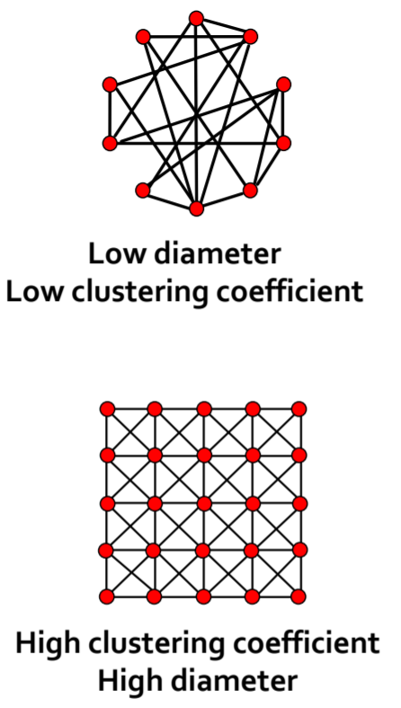
  • Diameter: The maximum shortest path length between any two nodes in a graph
  • Average Path Length: Sum of distances divided by the number of node pairs
• Clustering Coefficient: C

  • Measures the connectivity of a node's neighbors: Number of edges between neighbors divided by the node's degree:

    \[ C_{i}=\frac{2 e_{i}}{k_{i}\left(k_{i}-1\right)} \]

• Connected Components
  • The size of the largest component (giant component) is called connectivity, which is the number of nodes in the largest connected subgraph
• Random Graph Model

  • Viewing a graph as the result of a random process, with two parameters n and p: n total nodes, with edges independently established with probability p. Clearly, these two parameters are not sufficient to uniquely determine a graph. Consider its degree distribution, path length, and clustering coefficient

  • P(k):

    \[ P(k)=\left(\begin{array}{c} n-1 \\ k \end{array}\right) p^{k}(1-p)^{n-1-k} \]

  • h: Olog(n)

  • C:

    \[ =\frac{p \cdot k_{i}\left(k_{i}-1\right)}{k_{i}\left(k_{i}-1\right)}=p=\frac{\bar{k}}{n-1} \approx \frac{\bar{k}}{n} \]

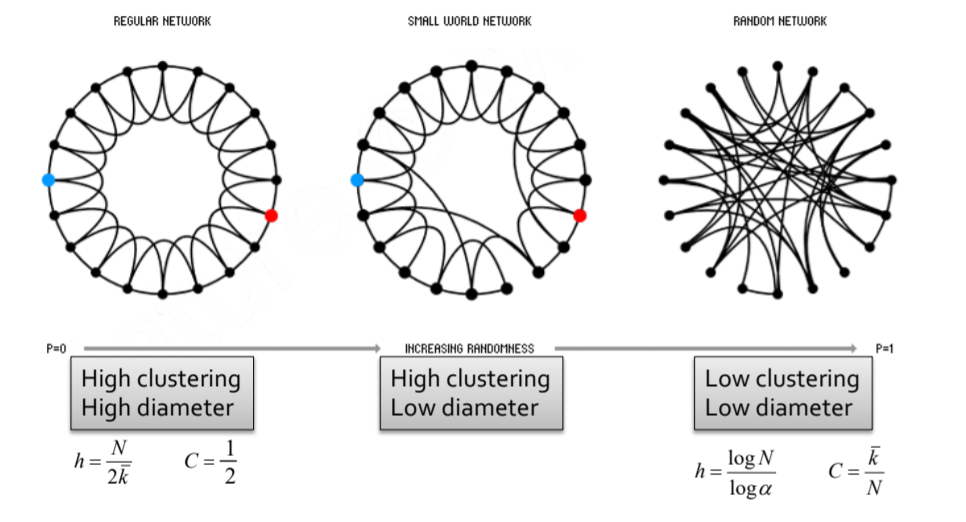
  • Connectivity: As p increases, the graph becomes increasingly likely to have connected subgraphs, specifically as follows:

• Small World Model
  • Maintaining a high clustering coefficient while having a short diameter
  • How to construct such a graph? Start with a high-clustering, long-diameter graph, and introduce shortcuts:
• Kronecker Graphs: Recursively generating large realistic graphs

Graph Features: Texture, Subgraphs, Small Graphs

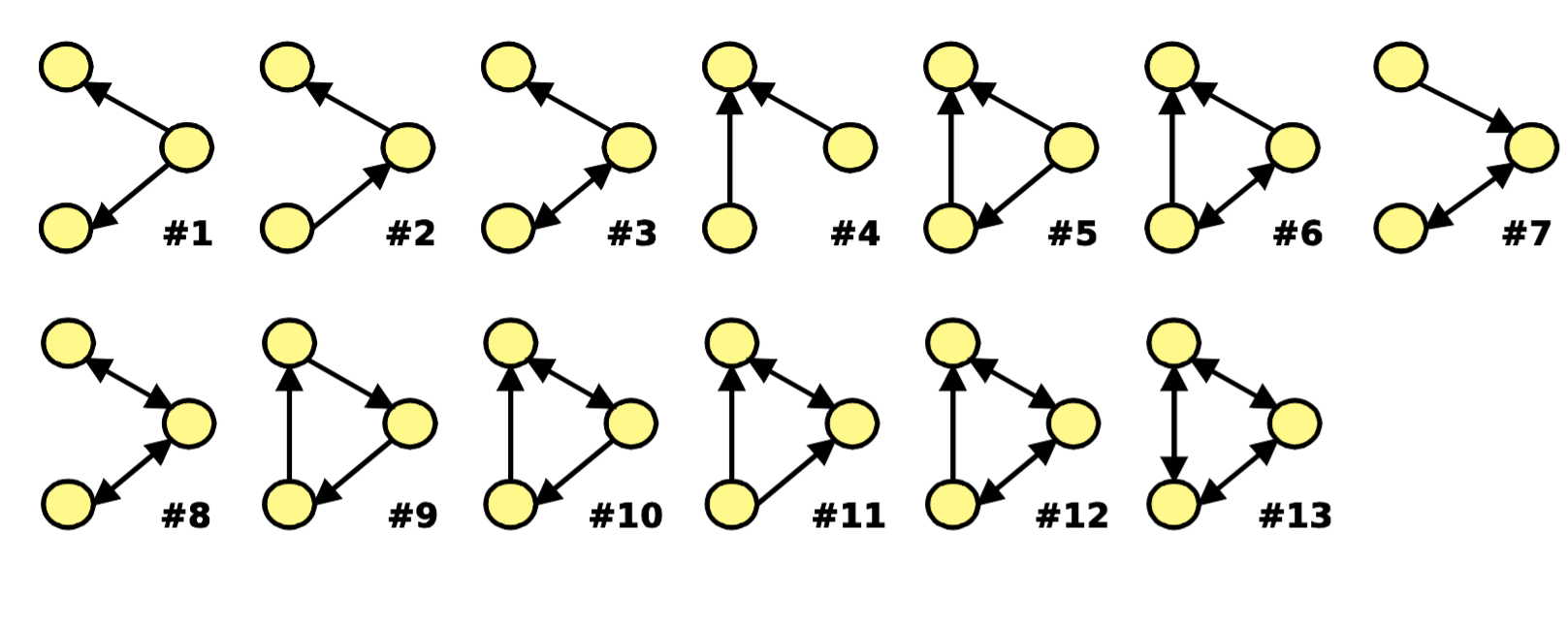
• Subgraphs, taking a three-node subgraph as an example:

• Assuming all nodes are identical, subgraphs focus on structural features of nodes and edges. If we define a significance for each subgraph, we can construct a feature vector.

• Defining Texture: Motifs, "recurring, significant patterns of interconnections", i.e., small induced subgraphs that appear frequently and are more significant than expected in randomly generated networks

• The significance of a motif can be defined by its occurrence ratio in real and random graphs:

  \[ Z_{i}=\left(N_{i}^{\mathrm{real}}-\bar{N}_{i}^{\mathrm{rand}}\right) / \operatorname{std}\left(N_{i}^{\mathrm{rand}}\right) \]

• RECAP Algorithm: Finding motifs in a graph

  • Based on the real graph, define a random graph with the same number of nodes, edges, and degree distribution
  • Find the significance of each subgraph in the real and corresponding random graphs. Subgraphs with high significance are motifs

• Graphlets: Node feature vectors

  • Graphlet Definition: Connected non-isomorphic subgraphs
  • In graphlets, we inject node-level features. For three nodes, there are only two graphlets: a triangle or a line connecting three points
  • In a triangle, each node is equivalent (relative to other nodes in the graphlet)
  • In a line, the two end nodes are equivalent, and the middle node is another type
  • Graphlets are very sparse: 11,716,571 types for n=10, not counting different node types

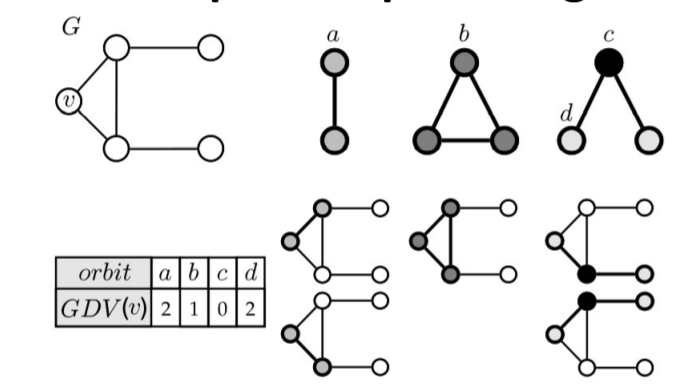
• Generalizing the degree concept, Graphlet Degree Vector (GDV) represents the graphlets a node touches, with each type occupying a feature and its value being the number of such graphlets touched:

• GDV measures the local topological state of a node

• Finding graphlets/motifs: Three types of algorithms

  • Exact Subgraph Enumeration (ESU) [Wernicke 2006]
  • Kavosh [Kashani et al. 2009]
  • Subgraph Sampling [Kashtan et al. 2004]

• Graph Isomorphism: How to determine if two graphs are topologically equivalent?

  • Defining Roles: The function of nodes determined by structural information
  • Roles can be defined as a collection of nodes with similar positions in a network
  • Difference from communities: Nodes in the same role do not necessarily need to be directly connected or have indirect interactions, but occupy the same position in the neighborhood structure
  • Structural equivalence: Nodes are structurally equivalent if they have the same relationships to all other nodes
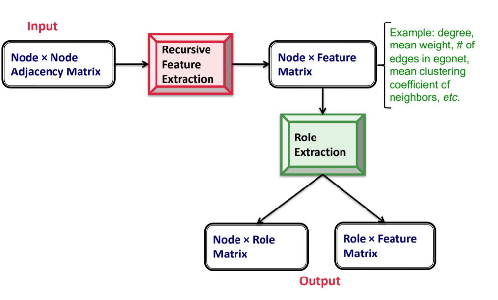
  • How to discover roles? ROIX algorithm
  • Recursive feature extraction: Construct base features, continuously aggregate and iterate, prune using correlation
  • Role extraction: Essentially matrix decomposition, viewing roles as latent topics. RolX uses non-negative matrix factorization for clustering, MDL for model selection, and KL divergence to measure likelihood

Spectral Clustering

• Three-step approach

  • Preprocessing: Obtain a matrix containing the entire graph's information
  • Decomposition: Perform eigenvalue decomposition, mapping each node to a low-dimensional embedding
  • Grouping: Cluster based on low-dimensional embedding

• Problem Definition: Graph partition, dividing graph nodes into mutually exclusive sets

• A good partition should maximize internal connections and minimize inter-set connections

• Define cut(A,B) as the sum of connection weights between nodes in sets A and B

• To consider internal connections, define vol(A) as the sum of node degrees within A

• Conductance metric:

  \[ \phi(A, B)=\frac{\operatorname{cut}(A, B)}{\min (\operatorname{vol}(A), \operatorname{vol}(B))} \]

• Finding a good partition is NP-hard

• Spectral-based partitioning details omitted for brevity due to mathematical complexity

• Spectral clustering approaches:

  • Preprocessing: Construct Laplacian matrix
  • Decomposition: Eigenvalue decomposition of L matrix
  • Grouping: Sort nodes by component values, find a split value
  • Visualization shows optimal splits correspond well to clustering
  • Two multi-class clustering methods:
    1. Iterative clustering
    2. K-class approach using k eigenvectors and k-means
  • Determine number of clusters by largest gap between k-th and (k-1)-th eigenvalues

• Motif-based spectral clustering

  • Upgrade edge concept to motifs
  • Construct a new graph based on motifs
  • Perform spectral clustering on the new graph

Message Passing and Node Classification

• Semi-supervised node classification in transductive learning
• Three techniques:
  • Relational classification
  • Iterative classification
  • Belief propagation
• Key relationships:
  • Homophily
  • Influence
  • Confounding
• Collective classification makes Markov assumptions
• Three approximate inference methods detailed
• Methods include relational classification, iterative classification, and belief propagation

Graph Representation Learning

• Unsupervised method to learn task-independent node features
• Framework similar to word embedding
• Similarity defined through various methods:
  • DeepWalk: Based on random walk sequences
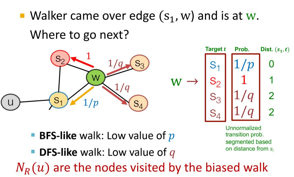
  • node2vec: Improved random walk strategy
  • TransE: Embedding for knowledge graphs
• Graph embedding techniques include:
  • Node-level averaging
  • Virtual node method
  • Anonymous Walk Embedding

Graph Neural Networks

• Introduce deep neural networks for graph encoding
• Key architectures:
  • GCN (Graph Convolutional Network)
  • GraphSage
  • Kipf GCN
  • GAT (Graph Attention Network)
• Training techniques:
  • Preprocessing tricks
  • Adam optimization
  • ReLU activation
  • No activation in output layer
  • Add bias to each layer

网络、随机图的属性

• degree distribution:P(k)
  • 即节点度的分布
• path length:h
  • path：即路径，可以与自己相交并通过同一条边多次
  • distance：两点之间最短路径
  • diameter：一个图的直径即该图上任意两点最短路径的最大值
  • average path length：distance之和除以节点对数量
• clustering coefficient:C

  • 衡量了节点的邻居的连接状况：邻居之间相连的边数除以节点的度：

    \[ C_{i}=\frac{2 e_{i}}{k_{i}\left(k_{i}-1\right)} \]

• connected components
  • largest component(giant component)的size称为connectivity，即最大连通子图的节点数
• Random Graph Model

  • 将图看成随机过程生成的结果，两个参数，n,p，即总共n个节点，每条边独立同分布按概率p建立，显然这两个参数不足以唯一确定一个图，考虑这样一个图上的degree distribution, path length以及clustering coefficient

  • P(k):

    \[ P(k)=\left(\begin{array}{c} n-1 \\ k \end{array}\right) p^{k}(1-p)^{n-1-k} \]

  • h:Olog(n)

  • C:

    \[ =\frac{p \cdot k_{i}\left(k_{i}-1\right)}{k_{i}\left(k_{i}-1\right)}=p=\frac{\bar{k}}{n-1} \approx \frac{\bar{k}}{n} \]

  • connectivity:随着p的增大，图越来越可能出现连接子图，具体如下：

• small world model
  • 在内聚程度很高的图上依然有很短的直径
  • 如何构造这样的图？首先以高内聚长直径的图作为起始图，在其中引入shortcut就可以了：
• Kronecker graphs：递归的产生 large realistic graphs

图的特征：纹理、子图、小图

• 子图，以三个节点构成的子图为例：

• 这里假设所有的节点都是相同的，子图只关注节点和边构成的结构特征。假如用一个significance来衡量每个子图，那么就可以构建一个feature vector。

• 定义纹理：motifs,“recurring, significant patterns of interconnections”，即图中出现很多次，具有显著程度（More frequent than expected, i.e., in randomly generated networks）的Small induced subgraph

• 通过某一个motifs在真实图和随机图中的出现次数之比就可以定义这个motifs的significance：

  \[ Z_{i}=\left(N_{i}^{\mathrm{real}}-\bar{N}_{i}^{\mathrm{rand}}\right) / \operatorname{std}\left(N_{i}^{\mathrm{rand}}\right) \]

• RECAP算法：找出一个图的motifs,

  • 根据真实图，定义一个随机图，其拥有和真实图一样的节点数、边数和度分布
  • 找出每一个子图在真实图和其对应的随机图上的significance，那么significance大的subgraph就是motifs

• 小图(graphlet)：节点特征向量,graphlet的定义：connected non-isomorphic subgraphs，在graphlet中，我们灌注node-level的特征，例如三个节点只有两种graphlet，即三角形或者一条直线连接三个点。在三角形中，每个节点是等价的（相对于graphlet中其他节点而言），而在一条直线中，两端的节点等价，中间的节点是另一类。graphlet非常稀疏，n=10的graphlet有11716571种，且不算其中不同类的节点。

• 将度的概念泛化，Graphlet degree vector（GDV）指一个节点接触到的graphlet，每一类占一个feature，值为接触到的这一类graphlet的数量：

• GDV衡量了节点的局部拓扑状态

• 寻找graphlet/motifs：三类算法

  • Exact subgraph enumeration (ESU) [Wernicke 2006]
  • Kavosh [Kashani et al. 2009]
  • Subgraph sampling [Kashtan et al. 2004]

• 图的同构：如何判断两个图是topologically equivalent的？

  • 定义roles:节点在图中所起的功能，通过结构信息来衡量，比如可以认为星型子图的中心节点具有相似的功能，或者直接归为一类功能，因此role也可以定义为A collection of nodes which have similar positions in a network。其和communities的区别：同一类role之间并不需要结构上互相连接或者有一定程度上的间接交互，而是他们在邻域结构内处于相同的位置
  • 那么可以定义节点级别的structurally equivalent: Nodes are structurally equivalent if they have the same relationships to all other nodes
  • 如何发现role?ROIX算法
  • recursive feature extraction：构建一些base feature，然后不断的aggregate不断的迭代，例如取mean，取sum，再通过相关性剪枝
  • role extraction，实际上是一个矩阵的分解，将role看成latent topic?：RolX uses non negative matrix factorization for clustering, MDL for model selection, and KL divergence to measure likelihood。

图谱聚类

• 三步走

  • 预处理：得到一个能够包含整图信息的矩阵
  • 分解：做特征分解，将每个节点映射到低维嵌入
  • 分组：根据低维嵌入做聚类

• 定义问题： graph partition，即将图的节点分为几个互不相交的集合，一个好的划分应该保证集合内节点之间的连接尽量多，集合之间节点之间的连接尽量少。

• 定义cut(A,B)为AB两个集合节点之间的连接权重之和，那么最小切就是使得cut(A,B)最小的AB划分

• 如何再考虑上AB集合内部的连接，定义vol(A)为A内部节点的度加权之和，那么可以得到衡量partition的一个指标Conductance：

  \[ \phi(A, B)=\frac{\operatorname{cut}(A, B)}{\min (\operatorname{vol}(A), \operatorname{vol}(B))} \]

• 找到一个好的partition是np-hard

• 基于图谱的划分：

  • 我们定义A为无向图的邻接矩阵，x为节点相关的向量，那么Ax得到就是邻域求和的结果

    \[ y_{i}=\sum_{j=1}^{n} A_{i j} x_{j}=\sum_{(i, j) \in E} x_{j} \]

  • 我们定义"spectrum of graph"，即图谱为A的特征向量构成的矩阵，按特征值\(\lambda\)大小排序，\(Ax=\lambda x\)

  • 那么假设图是d-regular，即所有节点的度都是d，那么很容易得到\(\lambda = d, x=(1,1,...,1)\)是该图的一组特征值/特征向量，且可以证明d是最大的特征值

  • 假如图是有两个连通分量，分别都是d-regular，那么对应的特征值依然是d，对应的特征向量有两个，分别是A分量里的节点置1，B置0以及vice versa

  • 这样根据node eigen vector的分量是1还是0就可以做一个划分，将节点分为两部分。显然两个d-regular的分量，用少数几条边连接起来，这应该是整图的一个好的划分。

  • 那么现在假设存在一个好的划分，整图是一个d-regular的图（这样两个分量就不是d-regular了，因为要考虑划分之间的连接所有节点的度才为d），分量之间有很少的连接。我们已知一个特征向量是全1的，且对应着最大的特征值d，那么直觉上第二大的特征值应该和d非常接近，因为我们知道断开的两个分量构成的图最大的特征值也为d，现在的图跟断开的图差别不是很大。而且由于特征向量之间相互正交而已知一个特征向量是全1，那么第二大的特征值对应的特征向量应该和为1，有正有负。类比于断开成两个分量的场景，我们也可以根据特征向量中分量的正负来划分节点。当然这都是直觉上的推测，下面引入Laplacian矩阵来详细说明。

  • 邻接矩阵的性质：n*n方阵，对称，n个实特征值，特征向量相互正交

  • 再定义度矩阵D，这是一个对角阵，第i个对角值存储第i个节点的度

  • 定义Laplacian矩阵，\(L=D-A\)，显然\(\lambda = 0, x=(1,1,...,1)\)是该图的一组特征值/特征向量。L矩阵的一些性质包括：

    • 所有特征值非负
    • 半正定
    • 可以分解为\(N^TN\)
    • 实际上三个性质是等价的

  • 那么L矩阵的二次型的含义是什么？

    \[ \begin{array}{l} x^{T} L x=\sum_{i, j=1}^{n} L_{i j} x_{i} x_{j}=\sum_{i, j=1}^{n}\left(D_{i j}-A_{i j}\right) x_{i} x_{j} \\ =\sum_{i} D_{i i} x_{i}^{2}-\sum_{(i, j) \in E} 2 x_{i} x_{j} \\ =\sum_{(i, j) \in E_{1}}\left(x_{i}^{2}+x_{j}^{2}-2 x_{i} x_{j}\right)=\sum_{(i, j) \in E}\left(x_{i}-x_{j}\right)^{2} \end{array} \]

  • 可以证明，二次型等价于矩阵的特征值加权x在对应特征向量上的坐标的平方求和

    \[ x = \sum _{i=1}^n \alpha _i w_i \\ x^TMx = \sum _i \lambda _i \alpha _i^2 \\ \]

  • 回到我们要找第二大的特征值，可以证明，对于对称阵：

    \[ \lambda_{2}=\min _{x: x^{T} w_{1}=0} \frac{x^{T} M x}{x^{T} x} \\ \left(\mathbf{w}_{1} \text { is eigenvector corresponding to } \lambda_{1}\right) \\ \]

  • 当这个对称阵是L矩阵时，有

    \[ \lambda _ 2 = min \frac{\sum _{i,j \in E}(x_i - x_j)^2}{\sum _i x_i^2} \\ \sum x_i = 0 \\ \]

  • 根据Fiedler'73的寻找最佳划分的方法，令节点label为1,-1来表示划分，所有节点求和为0来强制两个划分的集合大小一致，其提出的最佳划分是

    \[ \arg \min _{y \in\{-1,+1\}^{n}} f(y)=\sum_{(i, j) \in E}\left(y_{i}-y_{j}\right)^{2} \]

  • 可以发现将其label的限制从离散的1，-1放宽到实数值之后，等价于我们找L矩阵的第二大特征值和特征向量，第二特征值对应的特征向量分量的正负决定了划分情况（节点的分配情况）

• 回到spectral clustering

  • 预处理：构建L矩阵
  • 分解：对L矩阵做特征分解，得到每个节点在第二大特征值对应的特征向量上的分量
  • 分组：将节点按分量大小排序，找一个切分值，大于切分值的划为一组，小于切分值的划为一组。怎么找切分值？naive的方法就是设为0，expensive的方法就是都试一遍，取最好的
  • 通过可视化结果可以看到最优切分能够很好的对应聚类，而且多类也是一样，存在明显的分量差异：
  • 聚多类的两种方式：迭代式的聚类，每次聚两类；聚k类，找k个特征向量，而不仅仅是第二大的，然后相当于每个节点有k维特征，用k-means做聚类
  • 怎么确定聚几类？聚成k类时，第k大特征值和第k-1大特征值之间的差应该最大

• 基于motifs的spectral clustering

  • 当我们把边的概念升级到motifs时，就可以得到以motifs为特征的谱聚类
  • 同样的，我们可以得到基于motifs的Conductance，直接找也依然是NP-hard
  • 事实上，给定图G和motifs M，可以构建一个新图，在新图上做谱聚类即可
  • 定义新图为\(W\)，则\(W_{ij}^M\) = # times edge (i,j) participates in the motif M

消息传递和节点分类

• 在直推式学习中，已知图上部分节点的label，如何根据图的结构和已知节点，推断出其他节点的label？这就是半监督节点分类
• 三种技术：
  • Relational classification
  • Iterative classification
  • Belief propagation
• 关键在于利用网络（图）当中的关系（边），有三种重要的关系
  • Homophily: the tendency of individuals to associate and bond with similar others
  • Influence: social connections can influence the individual characteristics of a person
  • Confounding
• 最直观的想法，相邻的节点具有相似的label
• collective classification做出了马尔可夫假设，即节点的分类只受其一阶邻居影响
  • load classifier：不使用网络信息，先根据节点特征做出分类
  • relational classifier：学习到一个分类器，输入邻接节点的label和特征，输出中心节点的label
  • collective inference：不断的传播网络的相关性，对每个节点迭代的使用relational classifier
• 精确的推断是np-hard的，这里介绍三种近似推断的方法：

  • Relational classification：对邻域节点的label概率加权求和

    \[ P\left(Y_{i}=c\right)=\frac{1}{\sum_{(i, j) \in E} W(i, j)} \sum_{(i, j) \in E} W(i, j) P\left(Y_{j}=c\right) \]

    缺点：不保证收敛，且没有用到节点特征

  • Iterative classification：先对每个节点初始化一个特征向量，训练一个分类器（用有gold label的节点训练），输入特征向量输出Label，这是一个Local classifier，不考虑网络结构。等到每个节点都预测了label之后，根据网络结构进行消息传递，更新节点的特征向量，然后再用local classifier预测label,如此迭代。一篇应用论文REV2: Fraudulent User Prediction in Rating Platforms

  • Belief propagation：基于动态规划的方法，"Belief Propagation is a dynamic programming approach to answering conditional probability queries in a graphical model"

    • 定义label的矩阵\(\psi\),其定义了邻域节点label为i时，中心节点的label为j的概率\(\psi _{ij}\)
    • 给定每个节点的初始概率（先验）\(\phi\)
    • \(m_{i \rightarrow j}\left(Y_{j}\right)\)代表i到j的belief，即邻居i对于节点j的label为\(Y_j\)的估计
    • 则有： 即每次我们根据先验、label的转移概率、上一轮邻域节点的信念更新这一轮的信念；收敛之后根据先验和最终的邻域信念就可以推断中心节点的label
    • 参考论文：Netprobe: A Fast and Scalable System for Fraud Detection in Online Auction Networks Pandit et al., World Wide Web conference 2007

图表示学习

• 希望用无监督的方法学习到任务无关的节点通用特征
• 和word embedding一样，一个目标是，网络中相邻的节点，在embedding当中应该相似，因此框架是
  • 定义一个编码器，将节点编码成embedding
  • 定义一个节点相似度函数
  • 优化编码器参数，使得\(similarity(u,v) \approx z_v^Tz_u\)
• 最简单的方法：编码器只是一个embedding look up，每个节点预先分配一个embedding vector，例如DeepWalk,node2vec,TransE
• 因此主要区别在于如何定义similarity
• DeepWalk：
  • 每次随机游走采样出固定长序列，希望游走出发点和序列中的点比较相似，因此这里similarity定义为随机游走序列中的共现
  • 优化目标是softmax之后的log-likelihood，和word embedding一样，这里需要对所有节点计算来配分母，计算量太大，解决方案也是与word2vec类似，采用negative sampling，只采样部分负样本，用Noise Contrastive Estimation的目标函数来近似softmax之后的结果
  • 假如我们对所有节点无差别的sample出一个定长的随机游走序列，那就是DeepWalk模型
• node2vec
  • 同样是基于随机游走，node2vec在游走策略上做出了改进
  • 游走时不仅做dfs，还做bfs：前者获取Global macroscopic view；后者获取Local microscopic view
  • node2vec在两者之间做了插值，定义参数q为Moving outwards (DFS) vs. inwards (BFS)的比例，同时还定义了返回参数p，即返回到初始点
  • 具体的游走策略如下：
• TransE

  • 在知识图谱中，三元组(subject,predicate,object)表示了图中两个节点以及相连的边，都有feature vector

  • TransE的目标是学习到所有实体节点和关系边的embedding，该算法将边解释为一种翻译，即predicate将subject翻译为Object

  • 数学表示就是简单的\(u_{subject} + v_{predicate} = u_{object}\)

  • 训练采用了对比学习，采样负样本，用margin loss

    \[ \begin{aligned} &\sum \quad \nabla\left[\gamma+d(\boldsymbol{h}+\ell, \boldsymbol{t})-d\left(\boldsymbol{h}^{\prime}+\ell, \boldsymbol{t}^{\prime}\right)\right]_{+}\\ &\left((h, \ell, t),\left(h^{\prime}, \ell, t^{\prime}\right)\right) \in T_{\text {batch}} \quad \end{aligned} \]

• 如何embedding整张图？
  • 最简单的方法：学到节点的embedding，然后所有节点做平均或者求和
  • 或者引入一个虚节点，其和所有节点相连接，然后跑node-level embedding的方法，得到这个虚节点的embedding作为图的embedding，这种方法还可以得到子图的embedding
  • Anonymous Walk Embedding：我们将节点匿名，用其在随机游走学列中第一次出现的index来代表，那么长度为3的游走序列就有111，112，121，122，123五种可能。那么就可以：
    • 统计图中长度为l的所有序列，将图表示为匿名序列的特征向量，分量的值是该序列在图中出现的次数
    • 对每张图采样m个匿名序列，再统计特征向量
    • 学习到每个匿名序列的embedding，进而得到图的embedding。类似于语言模型，已知前n个匿名序列，预测第n+1个匿名序列，建立模型来学习参数

图神经网络

• 基于随机游走的方法其实是在similarity这部分做文章，在encoder这一块依然采用最简单的embedding lookup
• 图神经网络就为encoder引入了deep neural network
• GCN
  • idea：邻接关系定义了计算图，GCN利用图的结构来传播信息，更新节点的embedding
  • 通过aggregate邻域节点来生成node embedding，aggregate的过程使用神经网络，每一个节点基于其邻接状态定义了一个计算图
  • 最简单的aggregate：收集邻域节点的embedding，做平均，然后当前节点embedding和邻域平均embedding做拼接输入一个神经网络，获得当前节点下一层的embedding:
  • 这样就完成了encoder的定义，可以直接进行supervised learning，也可以接上random walks里的各种无监督目标函数来训练node embedding
  • 由于aggregate的参数在所有节点上共享，因此对于图上其他未知的节点也可以使用同一套encoder，新的一张图也可以。
• GraphSage
  • 在aggregate的形式上做了进一步扩展
  • 除了mean，其实任意的将多个embedding映射到一个embedding的函数都可以用来做聚合，例如pool，例如LSTM，
• Kipf GCN
  • 将每一层的aggregate&update操作写成矩阵形式，就可以利用高效的稀疏矩阵操作来提速
  • 其中的A都加了自环，邻域中包含了自己，而不是邻域与自己拼接，这里稍有不同。Kipf的形式其实是加权求和时权重做了对称归一化，考虑了邻域节点的度，而不仅仅考虑自身的度。
• GAT
  • 可以看到GCN和GraphSage在聚合邻域节点时，不同邻居节点的权重都是一样的，那么自然可以使用注意力机制，根据邻域节点和自身的embedding计算出注意力作为权重再聚合。
  • 参考transformer，使用multi-head attention
• GNN的训练技巧
  • 预处理很重要，Use renormalization tricks、 Variance-scaled initialization、 Network data whitening
  • adam优化，relu激活
  • output layer不需要激活
  • 每一层记得加bias