NLP Basics

Recorded some basic knowledge of deep learning learned when recording the seq2seq model in the entry-level NLP.

Neural Networks with Feedforward Architecture
When the dimensionality of the data is very high, the capacity of the sample space may be much greater than the number of training samples, leading to the curse of dimensionality.
Activation function. Used to represent the nonlinear transformation in neural networks. Without an activation function, if the neural network only has a weight matrix, it is a combination of linear transformations and remains a linear transformation. The use of nonlinear transformations can extract features that are convenient for linear transformations, avoiding the dimensionality disaster (?).
Softmax and sigmoid significance: Maximum entropy, convenient for differentiation, universal approximation theorem (with squeezing property)
Hidden layers can use the activation function ReLU, i.e., rectified linear, but the drawback is that it cannot use gradient learning to activate the function to 0 for the samples, so three extensions have been developed:
Absolute value rectification: right coefficient is -1; leakage rectification: right coefficient is fixed to a smaller value; parameterized rectification: coefficients are placed in the model for learning
Backpropagation
- Backpropagation calculates the parameter update values by determining the output biases through gradients, updating parameters layer by layer from the output layer to the input layer, propagating the gradients used by the previous layer, and utilizing the chain rule of calculus for vectors. The update amount for each layer = the Jacobian matrix of the current layer * the gradient of the previous layer.
- Backpropagation in Neural Networks:
![i0IIzT.png]() Initialize the gradient table. The last layer’s output calculates the gradient with respect to the output, so the initial value is 1. The loop proceeds from the end to the beginning, with the gradient table of the current layer being the product of the current layer’s Jacobian matrix and the gradient table of the previous layer (i.e., chain rule differentiation). The current layer uses the gradient table of the previous layer for calculation and storage, avoiding repeated calculations in the chain rule.
Initialize the gradient table. The last layer’s output calculates the gradient with respect to the output, so the initial value is 1. The loop proceeds from the end to the beginning, with the gradient table of the current layer being the product of the current layer’s Jacobian matrix and the gradient table of the previous layer (i.e., chain rule differentiation). The current layer uses the gradient table of the previous layer for calculation and storage, avoiding repeated calculations in the chain rule.
Recurrent Neural Network (RNN)
Recurrent Neural Network
Features: All hidden layers share parameters, treating hidden layers as state variables for convenient parameterization.
Using hyperbolic tangent as the hidden layer activation function
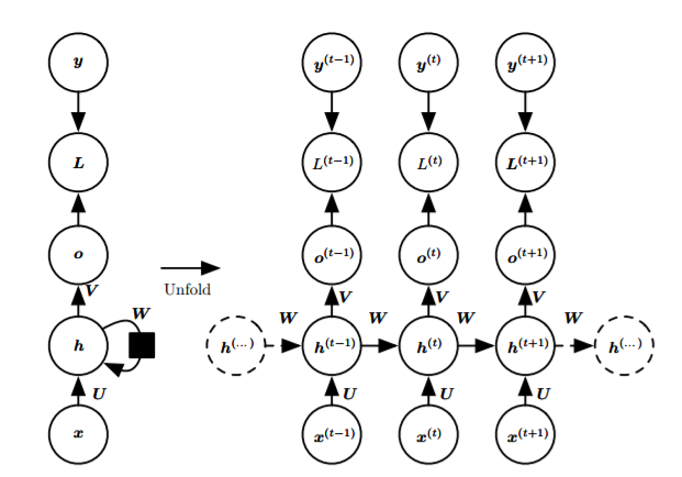
Input x, x passes through a weighted matrix and is activated by a hidden layer to obtain h, h passes through a weighted matrix to output o, the cost L, and o is activated by an output layer to obtain y
Basic Structure (Expanded and Non-Expanded):
![i0I7yF.png]()
Several variants:
- Each time step has an output, with recurrent connections between hidden layers:
![i0ITQU.png]()
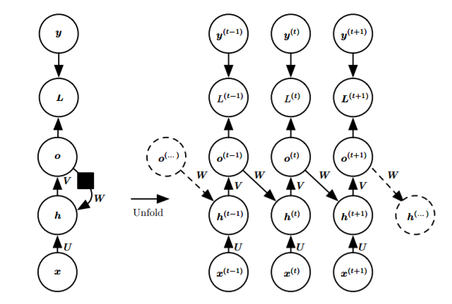
- Each time step has an output, and there is a recurrent connection between the output and the hidden layer:
![i0IqeJ.png]()
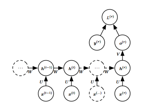
- Read the entire sequence and produce a single output:
![i0oCOe.png]()
- Each time step has an output, with recurrent connections between hidden layers:
Common forward propagation, softmax processing of output, negative log-likelihood as the loss function, and the cost of backpropagation through time is too high. Feedforward process:
Cost function:
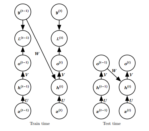
Replaced with the second RNN, using output-to-hidden layer loops, eliminating hidden-to-hidden layer loops, decoupling parallel(?), using a mentor-driven model (train the loop network W to the hidden layer with correct outputs, and use the actual output close to the correct output during testing) Mentor-driven model:
![i0ILw9.png]()
Bidirectional RNN
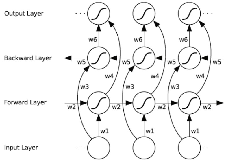
- Considering the dependency on future information, it is equivalent to the combination of two hidden layers
Sequence to sequence
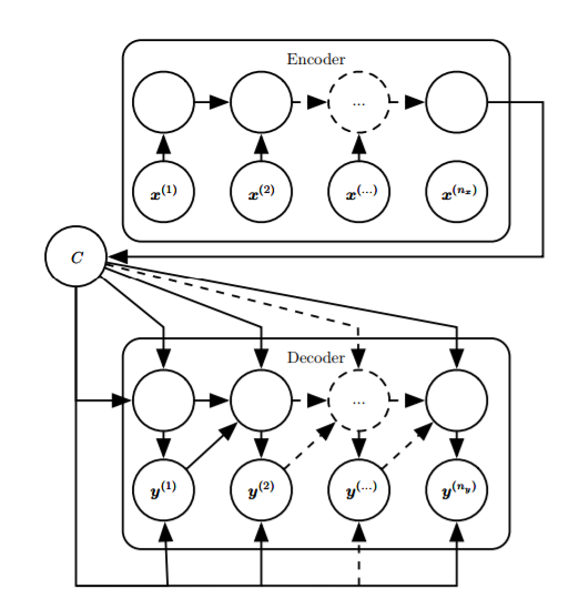
- Using encoders and decoders, it is possible to have different lengths for input and output sequences, generating representations (input sequences to vectors), and then generating sequences (a vector input mapped to a sequence). Sequence-to-sequence is a class of frameworks, and the specific models used by the encoder and decoder can be customized. For example, in machine translation, both the encoder and decoder can use LSTM. End-to-end models utilize the intermediate representation c, making the output depend only on the representation and the previously output sequence.
![i0IOoR.png]()
Deep RNN
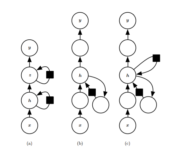
- A. Deepen the cyclic state, decomposing it into multiple hierarchical groups, i.e., deepen horizontally (hidden layer updates within a single cycle are performed multiple times)
- Introducing a neural network between input and hidden, hidden to output, and hidden to hidden, i.e., deepening the hidden layer states not only horizontally (time steps) but also vertically (a single training).
- C. Introducing skip connections to alleviate the path elongation effect caused by deepening the network
![i0IjF1.png]()
Long-term dependency problem in RNN
- Long-term dependency problem: As models become deeper, they lose the ability to learn previous information
- Perform eigenvalue decomposition on the weight matrix, repeatedly perform linear transformations, which is equivalent to matrix power operations, and the eigenvalues are also subjected to power operations. Eigenvalues with a magnitude greater than 1 will explode, and those less than 1 will disappear. A severely deviated gradient value can lead to a gradient cliff (learning a very large update). If it has exploded, the solution is to use gradient clipping, using the direction of the calculated gradient but limiting the size to within a small step length.
- It is best to avoid gradient explosion. In recurrent neural networks, transformations between hidden layers do not introduce nonlinear transformations, which is equivalent to performing power operations on the weight matrix, causing eigenvalues to explode or vanish, and correspondingly, the gradients of long-term interactions become exponentially small. Ways to avoid this include introducing skip connections in the time dimension (adding edges over long time spans), introducing leaky units (setting linear self-connected units with weights close to 1), and removing edges over short time spans (retaining only edges over long time spans).
Gated RNN
- Addressing the long-term dependency problem using a method similar to the leaky unit, gated RNNs, including LSTM and GRU, were introduced.
- Leakage Unit (?): We apply an update to µ(t) for certain v values as µ(t) ← αµ(t−1) + (1−α)v(t), accumulating a moving average µ(t), where α is an example of a linear self-connection from µ(t−1) to µ(t). When α approaches 1, the moving average can remember information for a long time in the past, while when α approaches 0, information about the past is quickly discarded. The hidden unit µ with linear self-connection can simulate the behavior of the moving average. This hidden unit is called a leakage unit.
Long Short-Term Memory
- LSTM: makes the weights of the self-recurrent connections context-dependent (gated control of the weights of this recurrence)
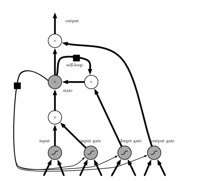
- LSTM modifies the hidden layer nodes (cells) in the ordinary RNN, with the internal structure as shown in the figure below:
![i0IvJx.png]()
- Visible in addition to the recurrent connections between cells in RNNs, there is an internal loop containing a forget gate control (how much to forget). The cell has an internal state s, which is different from the cell output h used for hidden layer updates between different time steps.
- All gate units have sigmoid nonlinearities, with input units being ordinary neurons that can use any nonlinear activation function.
- Three gates receive the same type of input, i.e., the current input x, the output of the cell at the previous time step h (not the internal state s), each having an independent weight matrix and bias. The outputs all pass through a sigmoid function to produce a value between 0 and 1, respectively representing the degree of memory of the current internal state s for the previous internal state, the degree of memory of the current internal state for the current input, and the degree of dependence of the current output on the current internal state of the cell.
- s: Updated internally based on two pieces of information: the previous internal state controlled by the forget gate, and the sum of the input controlled by the input gate and the cell output from the previous time step (not depicted in the figure?).
- Cell outputs h, the internal state overactivates the activation function, controlled by the output gate.
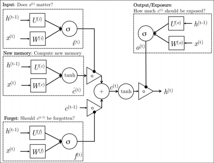
- Another more easily understandable figure:
![i0IxW6.png]()
Bidirectional LSTM
- As with bidirectional RNNs, each hidden layer node is an LSTM node, and there are no connections between the two hidden layer nodes in the bidirectional structure. Both hidden layers must be fully updated before the output layer can be computed, and the output at each time step depends on six weight matrices from w1 to w6.
- Because each output layer node receives the output of two hidden layer nodes, a processing step is required, and there are multiple ways to do this:
- Direct Connection (concat)
- Sum
![i0oSSK.png]()
Word embedding, Word2Vec
- Using the distributed representation of words (word embeddings or word vectors) to model natural language sequences, through the training of context-word pairs (one-hot vectors), a neural network is obtained, and the weight matrix from the input layer to the hidden layer is considered to contain all word vectors in the dictionary, i.e., the word vector matrix. At this point, by passing the individual one-hot word vectors through the neural network, a low-dimensional word embedding of this word can be obtained in the hidden layer with the help of the weight matrix (word vector matrix). Since word vectors are obtained as by-products of training with context-word pairs, the distances between word vectors in space have actual significance, i.e., words semantically related have vectors that are closer together. A problem with this generation method is the high dimensionality, because the output of the neural network is the word vector, which is reduced to a one-hot vector by softmax, representing the probability of each word. When the dictionary capacity is very large, this leads to a very large computational load in the final output layer. W2V is a practical scheme for generating word vectors, which optimizes the generation of word vectors based on the NLM model and solves the high-dimensional problem. It utilizes two optimization schemes:
- Hierarchical softmax: The output is no longer a probability vector of dictionary size, but a tree, with leaf nodes being words, internal nodes representing word groups, represented by conditional probabilities, and using a logistic regression model. W2V utilizes this model, eliminating the hidden layer, directly projecting the output of the projection layer into the tree, and improving the tree to a Huffman tree. Because the hidden layer is eliminated, W2V avoids large-scale matrix computations linearly related to the dictionary size from the projection layer to the hidden layer and from the hidden layer back to the output layer, but because the number of leaf nodes in the tree is still the same as the dictionary size, the final normalization computation of probabilities is still very costly.
- Important Sampling (?): This method reduces the computational load by reducing the gradients that need to be calculated during backpropagation. Each output word with the highest probability (positive phase) should contribute the most to the gradient, while the negative phase items with lower probabilities should contribute less. Therefore, instead of calculating the gradients for all negative phase items, a sampling of some is computed.
- Incomplete understanding of several simplification methods for the computation of softmax layers, to be improved. Recommended blog post: Technology | Series of Blogs on Word Embeddings Part 2: Comparison of Several Methods for Approximating Softmax in Language Modeling
Attention Mechanism
- In the seq2seq model, the information provided by the encoder is all compressed into an intermediate representation, i.e., the output of the hidden layer state at the last time step of the encoder, and the decoder decodes only based on this intermediate representation and the word decoded in the previous step. However, when there are many time steps in the encoder, the intermediate representation generally suffers from severe information loss, and to solve this problem, an attention mechanism is introduced.
- The actual performance of attention is to generate intermediate representations by weighted averaging over various time steps at the encoding end, rather than generating uniformly at the final step of the loop. The time steps at the encoding end with higher weights, which are referred to as the attention points, contribute more information to the decoding end.
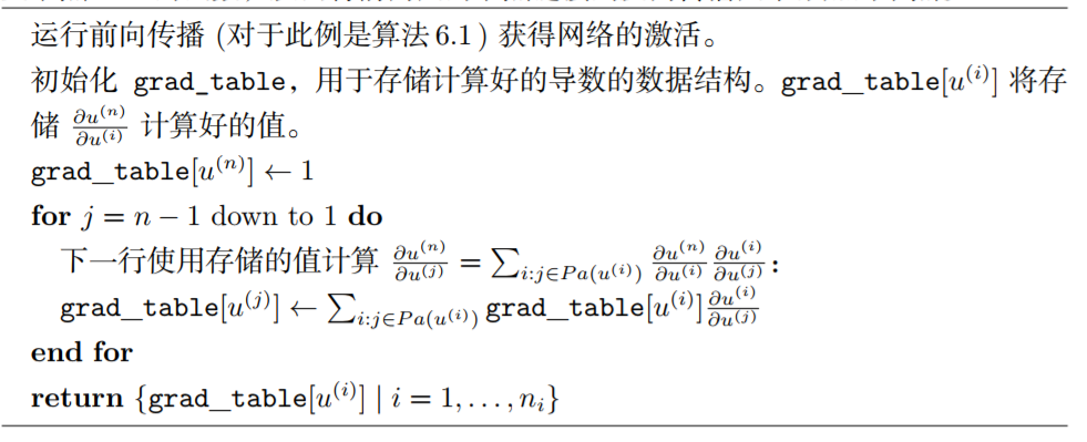 Initialize the gradient table. The last layer’s output calculates the gradient with respect to the output, so the initial value is 1. The loop proceeds from the end to the beginning, with the gradient table of the current layer being the product of the current layer’s Jacobian matrix and the gradient table of the previous layer (i.e., chain rule differentiation). The current layer uses the gradient table of the previous layer for calculation and storage, avoiding repeated calculations in the chain rule.
